Home / Tips & Tricks / How does the Reynolds Number affect my CFD model?

How does the Reynolds Number affect my CFD model?

The Reynolds number (Re) is the single most important non-dimensional number in fluid dynamics and is recommended to be calculated before you begin any new CFD modelling project.  The Reynolds Number is defined as the dimensionless ratio of the inertial forces to viscous forces and quantifies their relevance for the prescribed flow condition:

Re = \frac{\rho\cdot U_\infty\cdot L}{\mu}

Where U and L are the characteristic velocity and length scale of the problem, ρ  is the fluid density and μ is the dynamic viscosity. The use of the Reynolds number frequently arises when performing a dimensional analysis and is known as Reynolds principle of similarity. For example, air flow of U = 1 [m/s] over a flat plate of L = 1 [m] will exhibit the same flow pattern as air flow of U = 10 [m/s] over a flat plate of L = 0.1 [m]. This concept holds since the Re is equal and the flow is incompressible (i.e. the Mach number is low).

The Re also allows us to characterize whether a flow is laminar or turbulent. Laminar flow is characterized by lower Re and high diffusion over convection. Turbulent flow on the other hand is characterized by higher Re where inertial forces dominate considerably, resulting in largely chaotic flow. The flow may also undergo a transitioning phase whereby the flow exhibits neither completely laminar nor completely turbulent characteristics.

Free shear flow illustrating laminar, transition and turbulent phases


Note: Inertial forces are proportional to the square of velocity, while viscous forces vary linearly with velocity. Therefore as the Re → 0 it is reasonable to neglect convective terms (e.g. creeping flow). Similarly, as the Re → ∞ the viscous terms of the momentum equation can be neglected and the problem can be characterized purely by the generation of inertial forces (e.g. high supersonic and hypersonic flows).

For flows in a pipe of diameter L or non-circular pipes with hydraulic diameter L, empirical studies have shown that laminar flow occurs for ReL < 2500 and fully developed turbulent flow occurs for ReD > 4000. In the interval between, transition occurs. For external flows (e.g. flow over a flat plate), laminar flow is observed up to approximately ReD ~ 1×10⁵ to 5×10⁵ (where D is the distance from the leading edge) before transition to turbulence takes place and turbulent flow is observed thereafter.

Animation illustrating cyclic laminar vortex shedding


Factors influencing transition include roughness and local acceleration. The Turbulence Modelling team at ANSYS Inc, led by Dr. Florian Menter, have developed world-leading capabilities to allow CFD users to accurately model these transition effects. Using the Reynolds number, we can determine whether or not it is necessary to include transition in our simulation (as this may ultimately affect the development of the boundary layer). For example, for high speed flows over a flow plate, we may observe that the flow is predominately turbulent – in this case, transition may safely be neglected. Alternatively, for cases where laminar flow is observed for a large region of the geometry (i.e. low speed applications) then modelling fully turbulent flow may be an incorrect assumption.

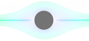
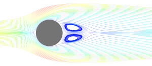
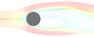
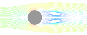
Consider the flow and wake pattern over a circular cylinder at various Reynolds numbers. At Re < 1 (see Figure 1), the flow is creeping and laminar and remains attached over the entire cylinder, which is a characteristic flow governed by momentum diffusion. At Re ~ 10 (see Figure 2) we begin to see a pair of stable and symmetrical laminar vortices in the wake. The flow in this regime is steady and the flow pattern will not change over time.

Figure 1: Re << 1 creeping flow (streamlines of velocity)


Figure 2: Re ~ 10 steady laminar flow (streamlines of velocity)


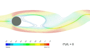
At a Re ~ 100 (see Figure 3) we see the development of a Kármán vortex street, whereby a repeating pattern of vortices are shed due to unsteady separation of the flow. While the flow is unsteady, the vortices are shed in a constant cyclic pattern and the flow remains laminar. A similar flow pattern is observed for Re ~ 105 (see Figure 4) with the exception that the flow remains laminar when it separates while the wake is largely unsteady and turbulent. In this case the use of a transition model is necessary. Assuming fully laminar flow will provide an erroneous pattern for the wake, and assuming fully turbulent flow will result in a delayed separation point (which affects the accuracy of lift and drag force prediction).

Figure 3: Re ~ 100 Kármán vortex street (streamlines of velocity)


Figure 4: Re ~ 1e5 laminar flow with largely unsteady and turbulent wake (Streamlines of turbulent kinetic energy)


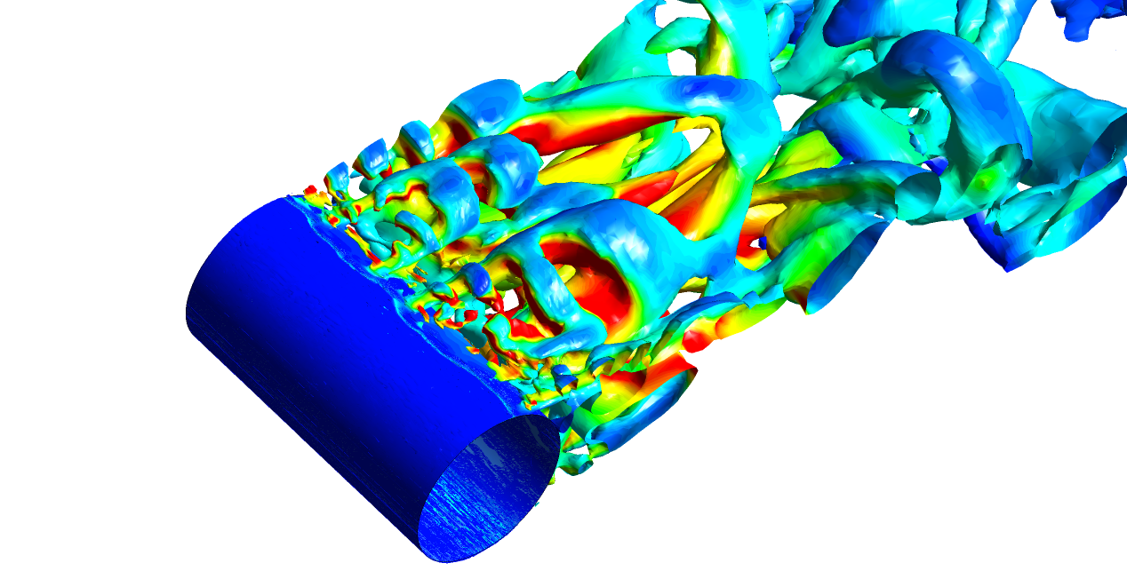
At Re ~ 106 (see Figure 5) the flow transitions to turbulence before it separates. The use of a transition model here is necessary to obtain correct viscous drag predictions but will ultimately not affect the point of separation and so we can assume that the influence of the laminar boundary layer is only additive. Furthermore, the flow can be approximated to be steady-state, as the delayed separation due to the higher stresses caused by turbulent fluctuations results in a narrower wake region. At even higher Re (while remaining incompressible - see Figure 6) a highly unsteady turbulent vortex sheet appears and instabilities in the boundary layer result in the separation point moving further upstream. This is called the trans-critical regime. This phenomenon must be captured using a high-order turbulent scale resolving simulation.

FIgure 5: Re ~ 1e6 steady fully turbulent flow field (streamlines of velocity)


Figure 6: Re ~ 5e6 three-dimensional trans-critical flow showing turbulent vortical structures


This small example should provide some basis for determining whether the use of a transition model is necessary, provided we calculate the characteristic Reynolds number and are aware of the flow pattern that we would like to capture. For further clarification, or for some insight into your own particular problem, please leave a comment below or alternatively contact our support line.


14 comments

  • I am a chem eng. student currently using ANSYS to study flow condition in reactors as part of my research. When you say transition are you referring to the transition sst turbulence model? Thank you! This blog is awesome!

    • In this post we are directly referring to the physics of laminar-to-turbulent transition. To capture this phenomenon, you can utilize either the transition SST model or the k-kl-omega model which are available in ANSYS CFD products. These models allow you to model both laminar and turbulent regions of the flow as well as the intermittent turbulence which is inherent with the physics of transition. These models are especially useful for aerodynamic flows where capturing the laminar and transitioning regions of the flow are crucial for accurate drag prediction

  • Hi,
    I am doing research work on fan, a pipe of 9 m long and the fan is located at 3 m from the inlet. I need to simulate the volume flow range from 2m3/s to 22m3/s.

    I have have done the simulation at design point with high Re model (k-epsilon), I got nice results. however I tried with komegaSST (low Re model). its taking massive amount of time when comparing to kepsilon, as well it is not converging fully.

    In my case how can I decide the turbulence model.
    I have done small calculation, at 2 m3/s the Reynolds number is 0.465*10^5 at design point (16 m3/s) 3.73*10^5.

    Thanks,
    Kumar

    • The choice of the turbulence model is problem dependent and will require generation of a suitable mesh. In your particular case SST with automatic wall treatment should work fine if the rest of the setup is correct. You may also be capturing transient behaviour, hence the (non)converging behaviour you have observed. You can investigate further by setting up additional monitors of interest for your problem (ie. quantified values such as pressure drop, forces on fan blades, minimums/maximums, etc...) and observing any transient oscillations in these monitors for your steady-state simulation. You can then test by reducing the pseudo-timestep used and re-running, then observe if this change also causes an associated change in the period of oscillation in the monitors. If it removes the oscillations, then it was a numerical issue. If it continues to oscillate, then it is likely to be an inherently transient and you need to run your simulation transiently (with a suitable timestep) instead of steady-state.

  • I am a physician in IVF
    I invented a new Needle for egg collection and I would greatful
    to come in mail contact with you.
    please see at You Tube Steiner Tan Needle
    My main question is: is it possible to categorize differnt needles
    ( single lumen, double lumen with Reynolds Number
    concerning capacity of flushing the egg out of follicles?
    Kind regards
    Hans-Peter Steiner, Graz, Austria

    • Thanks Hans-Peter for your interest. CFD can be used to evaluate the ability of different needle configurations (single, double lumen) to achieve these goals. If you don't have existing experience with CFD, we suggest in your case to contact CADFEM Austria in Vienna: http://www.cadfem.at and info@cadfem.at

  • Thanks for your tips. I am a physicist, just staring CFD simulations. How do we calculate Re beforehand, when we do not know the flow velocity. i.e. say I have a pipe and I know the inlet and outlet pressure values, but not inlet flow velocity.

    Also how do I calculate y+ beforehand and decide whether to use wall functions or resolve the boundary layer.
    Thanks in advance
    ramana

    • You can estimate both the likely flow velocities (for Re) and Y+ values beforehand, and then refine these calculations based on an initial CFD simulation. The decision to use wall functions or fully resolve the boundary layers is made in terms of the application (Re estimates, likely flow separation, whether or not conjugate heat transfer is important, etc) and the overall level of accuracy required.

  • Dear LEAP Support Team
    Thank you for your decent website. It is really helpful and useful especially for those who are new in CFD to get the great tips and tricks.
    I am simulating 2D-flow inside a rectangular channel with hiegh of 0.015 meter and length of 0. 400 meter at different velocity of flowing (0.4 m/s, ….,1.5 m/s). the flow is turbulent and I have been using K-e model (standard, Enhanced wall treatment,thermal effects). My goal is to find pressure drop throughout a rectangular channel. The amount of pressure drop changes with increasing of Re but it does not follow a consistent trend. For example when for Re=6000 I have dp= 18201.156 Pa
    and for Re=10000 I have dp= 4625.089 Pa
    and for Re=14000 I have dp= 195.99176 Pa
    and for Re=18000 I have dp= 1971.0658 Pa
    and for Re=22000 I have dp= 1959.609 Pa.
    I donot know why my results are incorrect.Please help me with detail explaining as I am new in CFD.
    thank you for your time and concern

    • It seems that you could benefit from some introductory training in CFD – this forum is aimed at addressing specific questions that users may have related to CFD best practice. How sure are you that a 2D channel is appropriately reflecting the experiment and that your residuals are fully converged at each design point?

    • Hi Ricardo, the value given by CFD-Post is the Turbulent Reynolds number. Also, because of the discretized nature of CFD, the more refined a mesh is, the more accurately the CFD solution will match empirical data.

  • Hello!
    Is it possible to estimate time required to complete model computation in ANSYS based on this model without any benchmark? I mean real time (in hours, days and so on).

Leave a Reply

Your email address will not be published. Required fields are marked *