Home / Tips & Tricks / Tips & Tricks: Convergence and Mesh Independence Study

Tips & Tricks: Convergence and Mesh Independence Study

RMS Residual Error Values

The previous posts have discussed the meshing requirements that we need to pay attention to for a valid result. It is important to remember that your solution is the numerical solution to the problem that you posed by defining your mesh and boundary conditions. The more accurate your mesh and boundary conditions, the more accurate your "converged" solution will be.


CONVERGENCE

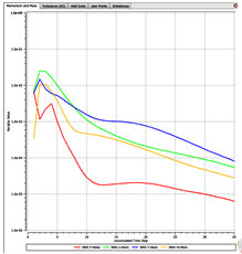
Convergence is something that all CFD Engineers talk about, but we must remember that the way we generally define convergence (by looking at Residual values) is only a small part of ensuring that we have a valid solution. For a Steady State simulation we need to ensure that the solution satisfies the following three conditions:


- Residual RMS Error values have reduced to an acceptable value (typically 10-4 or 10-5)

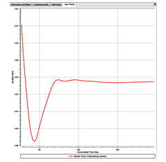
- Monitor points for our values of interest have reached a steady solution

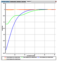
- The domain has imbalances of less than 1%.


RMS Residual Error Values

RMS Residual Error Values


Our values of interest are essentially the main outputs from our simulation, so pressure drop, forces, mass flow etc. We need to make sure that these have converged to a steady value otherwise if we let the simulation run for an additional 50 iterations then you would have a different result. Ensuring that these values have reached a steady solution means that you are basing your decisions on a single repeatable value.


Example of Monitoring a Value of Interest

Example of Monitoring a Value of Interest


As a rule, we must ensure that prior to starting a simulation we clearly define what our values of interest are, and we make sure that we monitor these to ensure that they reach a steady state. As previously highlighted, we also need to make sure that the Residual RMS Error values are to at least 10-4. Finally, we need to ensure that the overall imbalance in the domain is less than 1% for all variables.


Imbalances in the Domain

Imbalances in the Domain


MESH INDEPENDENCE STUDY

The approach outlined above results in a single solution for the given mesh that we have used. Although we are happy that this has "converged" based on RMS Error values, monitor points and imbalances, we need to make sure that the solution is also independent of the mesh resolution. Not checking this is a common cause of erroneous results in CFD, and this process should at least be carried out once for each type of problem that you deal with so that the next time a similar problem arises, you can apply the same mesh sizing. In this way you will have more confidence in your results.


The way we carry out a mesh independence study is fairly straight forward.


- Step 1

Run the initial simulation on your initial mesh and ensure convergence of residual error to 10-4, monitor points are steady, and imbalances below 1%. If not refine the mesh and repeat.


- Step 2

Once you have met the convergence criteria above for your first simulation, refine the mesh globally so that you have finer cells throughout the domain. Generally we would aim for around 1.5 times the initial mesh size.


Run the simulation and ensure that the residual error drops below 10-4, that the monitor points are steady, and that the imbalances are below 1%.


At this point you need to compare the monitor point values from Step 2 against the values from Step 1. If they are the same (within your own allowable tolerance), then the mesh at Step 1 was accurate enough to capture the result.


If the value at Step 2 is not within acceptable values of the Step 1 result, then this means that your solution is changing because of your mesh resolution, and hence the solution is not yet independent of the mesh. In this case you will need to move to Step 3.


- Step 3

Because your solution is changing with the refinement of mesh, you have not yet achieved a mesh independent solution. You need to refine the mesh more, and repeat the process until you have a solution that is independent of the mesh. You should then always use the smallest mesh that gives you this mesh independent solution (to reduce your simulation run time).


- Example

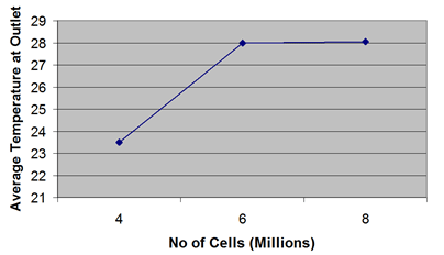
The best way to check for a mesh independent solution is to plot a graph of the resultant monitor value vs the number of cells in your simulation. This is illustrated below where we have three results from our steady monitor points for the average temperature at an outlet.


We can see that with 4 million cells we have a result, which could be "converged" for that particular mesh, with 10-4 residuals and imbalances below 1%. By increasing the mesh resolution to 6 million cells, we can see that there has been a jump in the value of interest that is not within my user specified tolerance (in this example I'll say +/-0.5 degrees).


By increasing the mesh size further we can see that the 8 million cell simulation results in a value that is within my acceptable range. This indicates that we have reached a solution value that is independent of the mesh resolution, and for further analysis we can use the 6 million cell case, as it will give us a result within the user defined tolerance.


 Example of Mesh Independence Study

Example of Mesh Independence Study


It is important that all CFD users follow these steps to ensure that you are reporting accurate simulation results. Please contact our Support Team if you have any further queries on this approach.


In the next blogs we will begin to discuss the importance of turbulence model selection.

40 comments

  • I'm trying to optimise my model(geometry) where; for example, I'm going to change the inlet diameter many times and I'll do mesh indepenance study for each inlet diameter. My question is about how I can reduce the number of simulations to reach mesh-independent solution? On other words, can I conduct only one mesh independance study when I use my maximum inlet diameter only and for the rest of inlet diameter values I can use the same number of elements for them.
    If not, is there any way to conduct mesh indepenance study more quickly in case of geometry optimisation?
    I'm looking to hear from you ASAP.
    CFX user

    • Hi Al,

      Thanks for your question.

      A bit of background… We conduct mesh independence studies in CFD to make sure that the results we get are due to the boundary conditions and physics used, not the mesh resolution. So if the results do not change with mesh density, we have achieved mesh independence. The issue is that this varies from case to case, depending on the physics involved and flow structures seen. So if we model the flow in a pipe with lots of bends and vary the radii of the bends, we can perform mesh independence studies on any of the configurations. But if we experience flow seperation around the bends as the radii decreases, we have a new flow structure, so a mesh that is indpendent at large corner radii may not be independent at smaller radii due to the flow structure change.

      With regards your case, as with any CFD case, it can be hard to get it right first go. You really need a good idea of the flow that you expect to see. If the changes in inlet diameter are not going to change the general flow structure, then mesh independence can be demonstrated on any of your configurations. If a change is expected, then it's good practice to model for the worst case scenario.

      Also, when doing independence studies, remember that cell volume varies with the third power of edge length. So there is no point increasing node count by 10% each time as this will equate to only a 2% change in edge length. Aim to at least double the mesh count each time, which still only give 25% change in edge length.

      Feel free to contact LEAP's support hotline if you have further questions.

      Thanks,

      LEAP Support

    • Hi again,,
      I'm trying to conduct mesh indepenace study for swirl flow induced by buoyancy.
      Only for one case, I cannot reach constant value of my intersted variables in some important regions within my domain or even at least having <1% differences. while I increase my mesh number, I reach my convergence criteria (1e-5 7 <0.01 for consevation target.
      I conduct my simulation using steady state mode.
      any comment can help.
      Regards
      CFX user

    • Hi Al,

      Thanks for this additional information.

      In general: When using the steady-state solver, we are asuming that the flow is not changing with time. If this assumption is not correct, we will possibly either experience periodic oscillations in our residuals, or periodic oscillations in our monitor points. This is a clear indication that the physics, geometry and/or boundary conditions of the setup dictate an unsteady flow. In this case you will need to activate the unsteady solver, which will allow the unsteady flow features to be correctly resolved by the solver.

      When using the unsteady solver in CFX you specify a timestep size. This must be small enough to capture the flow features of interest. Say you have a region where velocity is fluctuating at 5Hz. To correctly resolve a fluctuation you generally want approx 20 timesteps per cycle. Hence you will want a timestep of 0.01s or less. There may also be other flow features or physics in your simulation that require smaller timesteps, so just like with mesh independence studies, you will need to conduct a timestep independence study, whereby you test at increasingly small timesteps (dt = 0.01, 0.001, 0.0001, 0.00001, etc) until you meet the following criteria:
      Osciallations in fluid flows at monitor points are well resolved (`20 timesteps per oscillation) You reach good convergence at each timestep in around 5-10 iterations.

      In fact, there are more criteria for assessing the choice of timestep, which vary with the type of physics you are interested in. The ANSYS Fluent and CFX user guides have great information on this and are essential reading for anyone conducting an unsteady simulation. You must also consider how to post process your data (time averaging) and how to store your transient data during the simulation.

      Finally, a word on your specific case: flows involving buoyancy often do not exhibit a steady equilibirium and therefore require an unsteady solver and small timestep to resolve correctly.

      Hope this helps!

      LEAP Support

  • This is with reference to Fluent

    In a steady state simulation if a reduction of under relaxation factor (for pressure) and a reduction of time scale factor (pseudo transient algorithm) gives convergence with the monitor points then -

    Is it fine to relay on such convergence (or) is it always a must in general to
    run a few more iterations by revoking the default under relaxation factor
    and with a time scale factor = 1 ?

    It is a pressure based coupled solver in double precission with :
    pressure --> standard, momentum --> second order, turbulence --> first order, Energy equation not involved

    SST turbulence model with low-Re corrections disabled

    • Hi,

      The value specified for under-relaxation factors (segregated solver), or correspondingly the global Courant numbers/pseudo time-step (coupled solver) will not affect the final converged solution. This is also the case when you apply explicit relaxation to specific variables. It will however affect the time required to achieve convergence. So there is no need to set relaxation factors higher before obtaining a final converged solution.

      When using the pressure-based coupled solver, if you set the time-step (or correspondingly the Courant number) to be too high it may cause the residuals to hang and not converge, or in some cases may cause divergence. On the other hand setting the values too low will result in a slowly converging solution ultimately resulting in higher computing costs. You can estimate the time-step if you consider a characteristic length and velocity scale of your model. Alternatively you can start with a conservative value for the time-scale and appropriately adjust it as you monitor convergence.

  • Hi,i want to know which type of grid is better for 2D unsteady turbulent flow,it is structured or unstructured ,which type of cell,i am doing on vortex induced vibration on bluff body.can u please suggest me which type of meshing is better for my case.

    • Hi,

      There are benefits with adopting either a structured quadrilateral grid or an unstructured triangular mesh and ANSYS has tools which can be used for both. The questions to consider are the degree of sophistication of the modelling process and the complexity of the geometry. If the flow is aligned with the geometry and the geometry is not complex, then it is beneficial to adopt a high-quality quadrilateral grid, as you will reduce the overall cell count and you will produce less error due to numerical diffusion. If the flow is not aligned well with the geometry (which is generally a result of complexity in the geometry) then it may prove difficult to generate a quadrilateral mesh, and you may resort to a triangular grid. In this case, a high-quality triangular grid will produce a negligible difference in results with a quadrilateral grid, and the preparation time will be significantly reduced.

  • Hi,

    I am simulating channel flow with a very high flow in Fluent and I am using unsteady simulation. You write in this blogpost that for steady flow there are three conditions that must be satisfied for the solution to be converged for a steady state simulation. Are the same conditions applicable to an unsteady simulation? And what is meant by the residual RMS error values? Are those the values for the continuity equation, x-,y- and z-velocity, k and epsilon? (when running a k-epsilon turbulence model).

    Best Regards,
    Mira-Lisa

    • If you are using an unsteady simulation then you would expect to see a changing flow field over time and therefore your simulation will need to be time accurate. It accounts for this by solving the unsteady terms in the governing equations using an implicit second order backward time-stepping algorithm. The governing equations in CFD aim to satisfy the conservation laws of mass, momentum and energy. The RMS residuals give us the change in error from subsequent iterations (averaged over each cell) from solving algebraic forms of the conservation laws. At the start of the simulation, we might expect to have a large residual error and as we progressively iterate we will expect to see a decline in the residual error as the flow field converges. You can assess how the solver is satisfying the conservation laws by checking the domain imbalances (i.e. the mass, energy, etc. out – the mass, energy, etc. in). This is another methodology to assess global convergence, as we cannot safely assume the flow field is converged until these imbalances tend towards zero (and is especially evident for problems involving heat transfer, source terms and other complex physics). As you have suggested the more physics you implement, the more additional scalars need to be solved for. Hence a three dimensional turbulent problem involving heat transfer and a mixture of gases will solve for mass, momentum (in x, y and z directions) and energy, as well as for the additional scalars which account for the production and dissipation of turbulence and the mass fractions of the gas mixture. For your unsteady simulation, these need to be satisfied for each timestep.

    • So does this mean that I can use monitor points (in combination with the residuals and flux report) when showing that my unsteady solution has converged?
      Thank you for your help!

      Best regards,
      Mira-Lisa

  • Hello ,

    Thank you for your useful article,
    I have some questions that would appreciate if you answer them.

    - I have seen some discussion on the CFD-Online that suggests the Steady state time step(physical time step) should not be lower than the advective time step to ignore capturing the disturbances in the flow that cause residuals not to converge, if it is true how I can check the advective time step?

    - On the CFX manual I have read that physical time step can be set to the 1/3 of the flow residual time , and the residual time can be estimated on the post.P by checking the time of the stream line.Please let me know if I am correct.

    - CFX uses the implicit method , then it should not be so sensitive to the steady state time step , then why should we do the time step study?

    Thank you in advance

    • ANSYS CFX employs the so called False Transient. A timescale is used to move the solution towards the final answer. In a steady-state simulation the timescale provides relaxation of the equation in non-linearities . A steady-state simulation is a ‘transient’ evolution of the flow from the initial guess to the steady-state conditions

      The physical time step is the time represented in each iteration of the solution. CFX-Solver has the ability to calculate physical time step size for steady-state problems. If you do not know the time step size to set for your problem, you can use the Auto Timescale option.
      You can check the residence time either by having a look at the time on the streamlines or by dividing your volume by the volumetric flow rate. You want to know the time step in order to avoid having it too small (so that it takes a long time to have your solution to be calculated), or too large (that might cause convergence issues and it is not able to capture the characteristics of the phenomena you are studying).

  • This is a very interesting blog!

    I have a question about "Residual RMS Error values": How I can determine the acceptable values ​​for the RMS? Although normally RMS values ​​are 10-4 or 10-5, I've seen simulations in which values ​​10-3 or 10-2 are used.

    What is the criterion for choosing one value or another?. Is there any recommendation according to the problem considered?

    Best regards

    • There is no real precursor to determine what residual error values should be reduced to for acceptable convergence. This is because residual error may also reflect local areas of instability which is not representative of global convergence. We would advise that you monitor residual plots in conjunction with additional monitor points that reflect the convergence of a quantitative result of interest. For example, if you are performing an aerodynamic simulation, you may choose to monitor the convergence of the drag coefficient (along with the residuals) to judge convergence. Alternatively if you are performing an internal flow you may choose to monitor the pressure drop in your system. If you see that the monitor points have converged, but residuals are still oscillating due to small local regions of instability, we would likely accept the solution as a converged result.

  • Hello,

    Thank you for this article !

    I have a question regarding the mesh independance study. If a mesh independance analysis has been done with a steady-state flow, I wonder is the mesh independance study does still make sense when switching to a transient simulation for the same geometry. I know that I have to check the influence of the time step when performing my new simulations but if the independance is reached for a steady flow, is it for a transient one ?

    Thank you for your help.

    • Hi Brice, the validity of this approach is problem dependent. If the flow features in your initial steady state results are representative of the likely transient flow features, then you can confidently assume that your mesh fidelity is appropriate. If transient flow exhibits shedding or other flow features that were not present in the steady result, then you will need to use your judgement on mesh requirements (in many cases, dynamic mesh adaption can be very helpful in these transient cases where the final flow features are unpredictable). As with all simulations, you should continue to review your results in the context of your initial assumptions and adjust modelling inputs (such as mesh and boundary conditions) as needed.

  • Hi, I am trying to simulate a turbulent flux in a completely open valve, but the residual of continuity equation does not converge. I have tried changing my model (initially, I wanted to use the k-omega SST model) and I have found the best solution with the standard k-omega model. So, I thought that refining the mesh I would find a better solution! I have tried but the solution found is, actually, even worse!! The other residuals are in the order of 10-4 – 10-5, but the residual of continuity passes from 9*10-3 for the coarser mesh, to 5*10-2 for the refined one. The solution presents a mass imbalance of 10-5 on 50 kg/s. What do you think should I do to obtain a better solution? can I consider the solution converged even if the RMS of the continuity equation is so high?
    I would love to have any suggestions because I do not know how to proceed.
    Thanks

    Dave

    • Hi, if you are a Fluent user, you can try locally scaling the residuals to have better indication of convergence. What do your monitor points suggest? For example, monitoring the force in the streamwise direction over the valve wall would be a good indication of convergence. It is likely that you have picked up a small area of unsteadiness (e.g. small oscillating vortex), and as you gradually refine the mesh you are tending to refine the unstable region even more, hence the mass residuals do not converge in steady state. We recommend that you solve transiently and review the convergence behaviour.

  • Hi,
    This is a very interesting article,
    Actually, I'm simulating slug flow in a pipe and I want to perform mesh independence study, of course the phenomenon is unsteady. From the initial run with time step 0.005 sec the global residual monitor shows oscillation for x,y,z, energy, continuity and water in a range between 0.1 to .005 but the turbulent kinetic fluctuated between 1 to 30+. for improving the convergence I set lower value for under-relaxation factor for pressure, velocity, and turbulent k-omega. Do I need to perform time independence study to reach better convergence and after that start mesh independence study?

    I ran the analysis for 3 sec first and then for 8 sec, I realized a bit difference in the result. Do you think the total physical time will affect the results? if not, can I run the analysis for 3 sec in the mesh independence study and then generalize it for 8 sec?

    Regards

    • A model should only be considered converged if the 3 criteria described in this post have been met (residual targets achieved, monitor invariance, and mass balance). As the model is not currently converging, you need to the refine the mesh to the point where a convergent model is obtained and then perform a mesh independence study. Typically, the physics being modelled dictate the time-step to such a degree that if the time-steps are converging, the temporal discretisation is already sufficient. This, in effect, renders time-step independence a bit of a foregone conclusion. With regard to the relationship between total run times and mesh-independence, if there are regions of important physics or high-gradient areas that are changing location over time, then it is certainly possible that a 8s solution would require a different mesh than a 3s solution.

  • Hi,

    Thanks for useful comments and helps.

    I have question about y+ value,for transient aeroacoustic problem which y+ should be used?Could you please advise?

    • Hi Mustafa,
      For aeroacoustic problems, considering that you want to accurately predict surface pressure fluctuations for dipole source contribution, you should definitely aim for a y+ of 1.
      Regards,
      LEAP CFD Support

  • How are you doing?
    Hopefully, everyone is doing well!
    I want to ask you question, I would be very thankful for your answer!
    I am running Eddy dissipate concept models (EDC) for more than 10 real experimental data. The cold flow is converged easily.
    But the problem is the time for hot flow, it takes long time like around 10 days or more to converge and get solution as well results.
    What is the problem in your opinion? What can I do to solve this problem? Please, I need your experience to help me solving this issue.

    Thank you so much
    Hashim

    • Hi Hashim
      Converging combustion problems can be very difficult at times, due to the high coupling between the flow/turbulence, energy due to reaction heat release, radiation, particle tracking, etc. Our advice would be to first converge the cold flow simulation, and then progressively ramp up the physics and high-order discretization in your simulation to give you better stability in convergence. For example, you can begin with cold flow in first order, then couple reactions (again using low-order discretization), then add higher-order discretization, and finally radiation. Additionally, residuals are very ambiguous and will not accurately report global convergence of your model. I would suggest the use of monitor points wherever possible to judge convergence.
      Regards,
      LEAP CFD Support

  • Hi LEAP,
    I'm running an unsteady state simulation about hot water charging process in a stratified thermal storage tank, and I have a problem. The mass & energy imbalance are still too high until 30 mins of charging process, though the majority of residuals has converged. Whereas I've tried to run it with steady state simulation before, and the mass & energy imbalance were <1%. My question is: does unsteady state simulation has effect on mass & energy balance?

    Thanks,

    Yogi

    • Hi Yogi,
      If anything an unsteady simulation should assist in convergence as the unsteady term in the scalar transport equations aims to provide additional stability to the simulation process. Can you comment on your convergence dependency on the time-step size? To ensure a more stable solution (especially given your application) you can try use adaptive time-stepping. This method will allow you to select a range of local cell Courant number for your domain, and will implicitly determine your time-step size to give the solution greater stability in convergence.
      Regards,
      LEAP CFD Support

  • Hi LEAP Team,

    Thanks for the interesting article.

    I have a question concerning mesh independence studies:

    As far as I know, a properly done mesh independence study requires a uniform and consistent refinement of the whole mesh (i.e. every region should be refined by the same factor and the quality of the mesh should at least remain constant). How can I achieve a uniform and consistent refinement for a unstructured and non-uniform mesh (with inflation layers), e.g. in ANSYS Meshing (i.e. how should the meshing parameters be adjusted in order to achieve a uniform and consistent grid refinement)?

    I would really appreciate if you could give me some hints concerning the question above or refer me to some reference which could help! Thanks in advance!

    Regards,
    Markus

    • If you have only used Global controls in ANSYS Meshing, you can use the Relevance slider to refine your mesh accordingly. If you specified body/surface/edge sizes, you can obviously alter those directly. For inflation layers, if you used aspect ratio, the cell heights should update appropriately as they will be directly related to the size of the underlying surface mesh. A first layer thickness specification would operate like the body/surface/edge sizes.

  • Dear LEAP team,
    We are performing CFD studies of an automotive geometry in a wind tunnel. We monitor drag and lift. We solve steady state with k-omega STT but in reality the flow field is transient and as a result the residuals do not drop. We average drag and lift over many iterations after the residuals reach the plateau, as much as 15 or 20 thousand.
    We also perform mesh independence studies by refining the mesh from coarse to medium to fine. However we do not reach a nice convergence of drag and lift as in the plot you show. Cl for example may increase from coarse to medium and then decrease to fine mesh.
    I have read somewhere that too fine meshes in steady state RANS may lead to problems.
    Could you please comment on this?
    Thanks!

    • In the absence of experimental data with which to compare your results, it can be difficult to have confidence or draw conclusions about a simulation for which the typical marks of convergence (target residuals met, steady-state behaviour of solution monitors, and mass imbalance <~2%) have not met. These hallmarks are certainly the recommended approach to judging convergence. Refining a mesh will capture the modelled physics with increasing fidelity. For a turbulent model, this means capturing an increasing amount of the transient behaviour in the system, which certainly causes convergence difficulty for a steady-state solver. If high fidelity of turbulent flow is required, a transient solution is usually a corollary. See Section 15.4.1 in the CFX Modeling Guide or 28.13 in the Fluent User’s guide for additional details.

  • Mahmoud Eslami Pirharati

    Thank you for your useful information,
    I have a question regarding mesh independence study in transient simulation.
    My Master's thesis title is ''CFD simulation for Newtonian fluids in packed bed with Finite volume method'' and i have to simulate in steady and unsteady conditions to compare pressure drop.
    As you know, the simulation regarding transient condition takes a lot and also mesh independence study would be time-consuming.
    If i check mesh independence in steady condition, is it also valid for transient condition? or I have to do it again for transient simulation?

    • Hi Mahmoud,
      A mesh independence check is something every CFD engineer should complete prior to the final solution. When a problem involves both a steady and unsteady component to the simulation, the answer to your question becomes dependant on whether there are any large, inherently transient phenomena occurring (e.g. shock waves, free surface etc.). If the problem is simple flow over a bluff body for both the steady state and transient simulations, you could assume the steady state mesh check to be suitable, however if the flow deviates largely from the steady state solution, then a mesh independence study is going to be beneficial. It is always good practice to review whether the results achieved are physical after each simulation, regardless of whether the simulation was steady, or unsteady.

      Thanks,
      LEAP Support

  • Hi,LEAP TEAM
    Thanks for this interesting article.
    But i have some questions in my mind and it will be very helpful if you kindly answer them.
    How will i do mesh independency test in ansys fluent? Specifically,what tools should be used? Should I refine mesh globally or locally?

    • Hi Ifti,

      Mesh independence is a very important concept to grasp as it can be used to distinguish whether the solution we are getting is independent of the mesh resolution. It also allows the user to ensure they are achieving the optimal solution time; and not enlarging their mesh and solution times.

      The best method to implement a mesh independence check is to gradually refine and coarsen the mesh in the important regions; and then compare the final results and plot their difference. Ideally you are looking to achieve a value that does not overly change, without over-refining the mesh. As we have mentioned before; finding the balance between mesh density and the final solution is crucially important to a CFD simulation and a mesh independence study is the first step to evaluating the accuracy of our results.

      Thanks,
      LEAP Support

  • Hi team,
    i am very impressed with all the discussions.
    my question is
    1) for the industrial purpose, we need immediate results in order to save time and cost. so, in such situations can we consider unconverged solutions for the presentation purpose while the exact values of parameters are not my priority.

  • VERY NICE AND SUPER RELEVANT DISCUSSION! I HAVE A QUESTION ABOUT THE y+ VALUE IN THE MESH INDEPENDENCY STUDY:

    - SHOULD WE PERFORM THE ENTIRE MESH INDEPENDENCE STUDY AND THEN AFTER THE GLOBAL NUMBER OF ELEMENT HAD BEEN CHOSEN ADJUST THE MESH IN A WAY THAT THE y+ MATCHES THE TURBULENCE MODEL USED?

    OR

    - SHOULD WE ANALYSE AND ADJUST THE y+ VALUE IN EVERY MESH SIZE PERFORMED IN THE MESH INDEPENDENCE STUDY?

    THANKS, A LOT LEAP SUPPORT TEAM!!

  • Thank you for the valuable content.

    I want to draw a flowchart for the process.
    Could you please let me know
    should I draw "mesh refinement" step before "mesh independence study" step
    or
    "mesh independence study" step before "mesh refinement" step?

    Best
    Tom

Leave a Reply to Bhawesh - Cancel Reply

Your email address will not be published. Required fields are marked *