
Engineers are continually under pressure to improve the performance of their products and often look to gain an edge using optimisation techniques. Whether they need to reduce drag along with increasing lift (or downforce) in external flows, or reduce pressure losses in internal flows, engineers historically relied on intuition to make geometry changes to achieve improvements over their existing designs (most often built using a parametric CAD approach). In recent releases, ANSYS Fluent has included a new feature called the Adjoint solver which allows engineers to optimize their products semi-automatically using results obtained from the CFD analysis.
What is the Adjoint Solver?
The Adjoint Solver is a specialized CFD tool that allows the users to obtain detailed sensitivity data for the performance of a fluid dynamic system. Designers can use this sensitivity data to automatically generate get an answer to the question “How and where should I modify my geometry to achieve my design objectives - ie. to reduce drag by 10% and/or increase lift by 10%?”. The Adjoint solver identifies the local geometry which needs to be modified and calculates the extent of the deformations needed to achieve these objectives. Using this approach, the ANSYS Fluent Adjoint solver offers the ability to develop products in a much more organic way than has previously been available to the designers.
Adjoint Server Workflow
The Adjoint solver allows the user to choose a “flow observable”, like lift or drag on a given surface, pressure drop between inlets and outlets, without the need for a typical design of experiments (DOE) study or the requirement to set several parameters to the model. The Adjoint solver will compute the derivative of these observable with respect to all the inputs of the system such as surface mesh, interior mesh, boundary conditions, material properties etc. These derivatives identify the regions of the domain where the defined observable is most sensitive to. Making changes in these sensitive regions will lead to changes in the observable. This is essentially the opposite of the traditional approach where we would modify each of these parameters one at a time and monitor the changes in our variables of interest.
Let us understand a bit more about how to use the Adjoint solver within ANSYS Fluent in this section. The overall Adjoint solver workflow is defined below:
- Run the initial CFD simulation until fully converged
- Setup Adjoint variable of interest named as observables.
- Specify appropriate Adjoint solution controls and solve the Adjoint problem.
- Post-process the solution to visualise sensitivities of the domain for the selected observable.
- Use design tool to find optimal design change that satisfies one or more goals or constraints provided.
- Define the region for the design change in accordance to design constraints.
- Specify Target/Reference change of the desired observable (increase or reduce from baseline value by 10%).
- Determine regions for Mesh Morphing and preview estimates for changes in the variable of interest
- Deform the mesh to achieve the required change in the variable of interest.
- Rerun the full flow simulation on the deformed mesh
- Repeat as necessary until user is satisfied with the final morphed geometry
- Use deformed geometry as basis for final component design (Option to export optimized 3D CAD geometry to SpaceClaim).
Application to an example
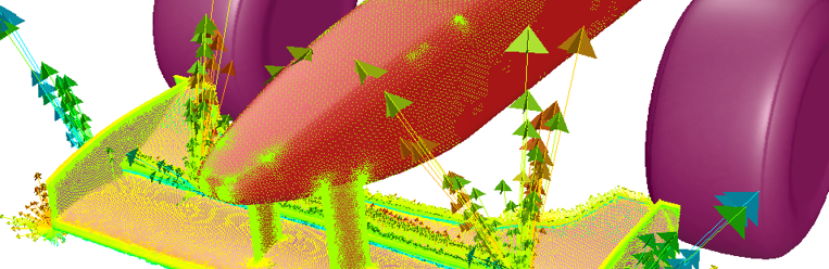
Let us see how to analyse the data produced by the Adjoint solver by looking at a simple example below. In the this example, we have chosen Drag as our variable of interest and the resulting shape sensitivity vectors are telling us the direction, and the relative magnitude we need to modify the geometry to increase the Drag of this airfoil. (In most cases we aim to reduce the drag of an airfoil so we would do the opposite!). The sensitivity vectors indicate that thickening the airfoil would increase drag. The results of the Adjoint Solver are thus quite intuitive to understand.
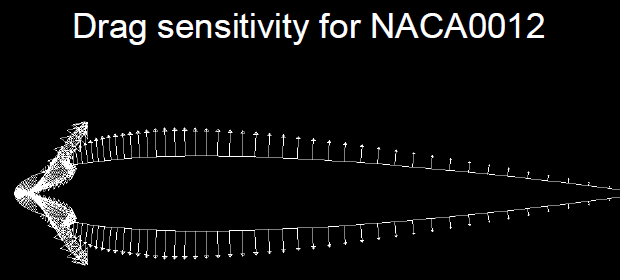
Fig. 1: Drag Sensitivity for NACA 0012
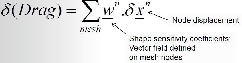
Fig. 2: Formula to determine change in drag from node displacements and shape sensitivity coefficients
Another key feature of the solver is its ability to estimate the change in drag produced by the airfoil due to the geometric changes made by the solver. This is done by summing up the sensitivities at each node multiplied by the displacement at each node as per the equation above. We can use this information to determine the exact deformations needed on the airfoil to achieve the required drag force. The whole process can be repeated for a few cycles to gain significant performance improvements on the baseline designs.
Now let's look at a more realistic Industrial application of the Adjoint solver. Consider a typical airfoil geometry used in wind turbines. In Fig 3, we can see that the adjustment of the variable of interest and the scale factor (seen as positive or negative values in the top line), results in variations in geometries and in the final efficiency of the airfoil.

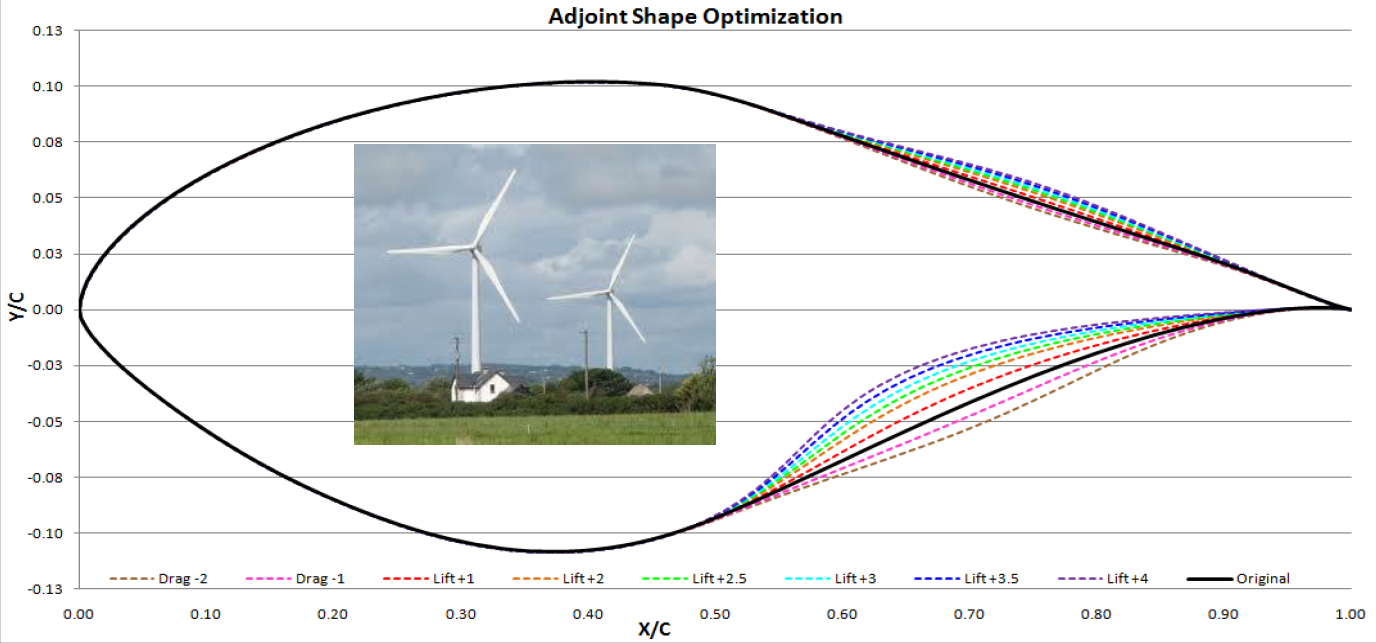
Fig. 3: Results for deforming geometry at trailing edge of wind turbine
In this exercise, the Adjoint solver was used to increase the performance of the wind turbine by improving the L/D ratio of the airfoil section from 7.97 in the baseline to 13.02 in the Lift+2.5 configuration. This is an increase of 63.36% which should lead to significant improvement in the electricity produced by the wind turbines.
Conclusion and next steps
As CFD engineers, it is worth understanding the advantages offered by the Adjoint solver over other more traditional optimisation techniques available in the ANSYS suite. Parametric optimisation is usually constrained by the way in the original CAD was built. Parametric optimisation only allows the user to change major geometric features like lengths, angles or radii. The Adjoint solver is is a uniquely different approach which considers localised changes which are de-coupled from the original parametric CAD, something akin to the ways in which topological optimisation is used in FEA (which can reduce the overall mass of a design by make subtle modifications to the geometry to achieve required structural performance improvements based on local stress/strain results). The advantage of the adjoint solver is that it can come up with very smooth and organic looking shapes - which often have a certain beauty which you don’t often see in engineering designs!
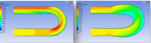
Fig. 4: Shape Optimisation of pipe bend using the Adjoint solver
This concludes the first part of our series on the ANSYS Fluent Adjoint solver. Stay tuned as we will follow up with a deeper-dive into some of the new and more useful features now available for the Adjoint solver to tackle more complex, real-world problems.


