Home / Featured / Turbulence Part 4 - Reviewing how well you have resolved the Boundary Layer

Turbulence Part 4 - Reviewing how well you have resolved the Boundary Layer

In recent posts we have comprehensively discussed inflation meshing requirements for resolving or modeling wall-bounded flow effects due to the turbulent boundary layer. We have identified the y-plus value as the critical parameter for inflation meshing requirements, since it allows us to determine whether our first cell resides within the laminar sub-layer, or the logarithmic region. We can then select the most suitable turbulence model based on this value. Whilst this theoretical knowledge is important regarding composite regions of the turbulent boundary layer and how it relates to y-plus values, it is also useful to conduct a final check during post-processing to ensure we have an adequate number of prism layers to fully capture the turbulent boundary layer profile, based on the turbulence model used (or more precisely, whether we aim to resolve the boundary layer profile, or utilize a wall function approach). In certain cases, slightly larger y-plus values can be tolerated if the boundary layer resolution is sufficient.

How can I check in CFD-Post that I have adequately resolved the boundary layer?

For the majority of industrial cases, it is recommended to use the two-equation turbulence models, or models which utilize the turbulent viscosity concept and the turbulent viscosity ratio (i.e. the turbulent viscosity over the molecular viscosity). We can make use of this concept to visualize the composite regions of the turbulent boundary layer, and ultimately visualize how well we are resolving the boundary layer profile. Consider the conceptual case-study of the turbulent flow over an arbitrarily curved wall. Prism layers are used for inflation, and tetra elements in the free-stream. Once we have calculated the solution, within CFD-Post we can create an additional variable for the eddy viscosity ratio. Then by plotting this variable on a suitable plane, and superimposing our mesh in the near-wall region, we can visualize the boundary layer resolution.

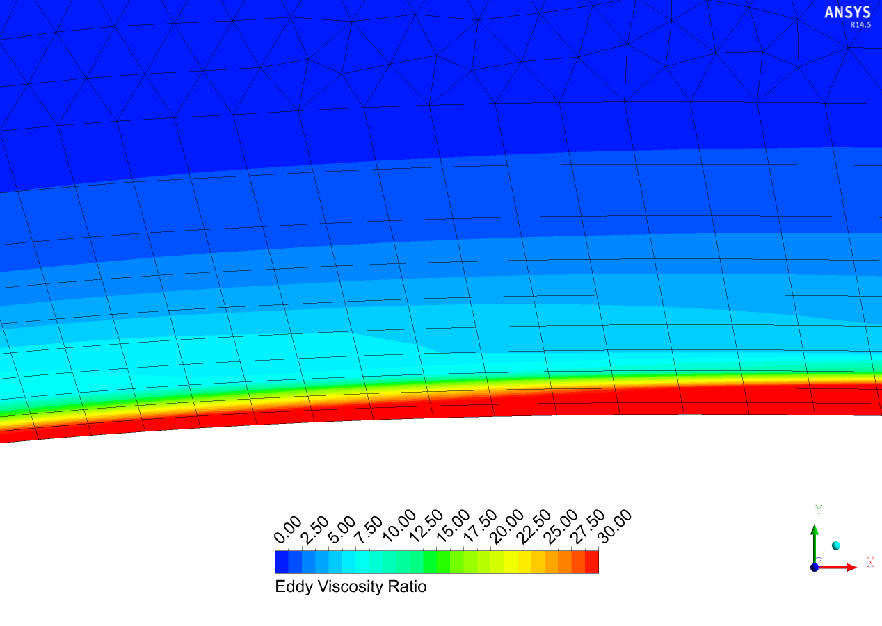
Figure 1: RKE with standard wall function – y-plus of 75 with 10 prism layers


Figure 1 provides an example of a reasonable wall function mesh. There is a good cell transition from the prisms to the free stream tetra elements. The y-plus we have prescribed at the first cell indicates we are in the logarithmic composite region of the turbulent boundary region, which is the region largely dominated by inertial forces and thus we have high levels of turbulence. The turbulence gradually dissipates as we approach free stream conditions (where the levels of turbulence are governed by inlet conditions), which is expected. At this stage, we could even reduce the number of cells in the inflation layer as we are clearly capturing the logarithmic region layer before approaching the free stream. Correspondingly, we could aim to reduce the y-plus value (y-plus ~ 20) to better capture the increase in turbulent viscosity as we move from the inner layer to the outer layer of the logarithmic region.

Figure 2: SST low-Re model – y-plus of 1 with 20 prism layers


Figure 2 provides a good mesh for a low-Re turbulence model. We observe that the transition in size from the final prism layer to the free stream tetra elements has been regulated well. Since we have prescribed a y-plus value of 1 we are within the laminar sub-layer, which exhibits laminar flow characteristics (thereby resulting in no turbulent viscosity). As we gradually move through the buffer region and into the logarithmic region we see a large rise in the viscosity ratio before it dissipates into the free stream. This maximum value will generally occur near the middle of the boundary layer, which also gives us an indication of the physical boundary layer thickness (twice the location of the maximum eddy viscosity ratio gives the boundary layer edge). As per the example given in Figure 2, it is essential that the prism layer is thicker than the boundary layer as otherwise there is a danger that the prism layer confines the growth of the boundary layer.

Figure 3: SST low-Re model – y-plus of 0.25 with 20 prism layers


Figure 3 ia an example of a poor quality mesh for a low-Re turbulence model (such as SST k-omega). In this case we have unnecessarily prescribed a very low y-plus value yet we have not compensated by appropriately allowing for more prism layers in the inflation layer. Therefore, we are capturing the laminar sub-layer to an excessive detail, and the boundary layer does not transition to the logarithmic region until we are well inside the free stream. Consequently there are cells which are not aligned with the direction of the flow and thus our boundary layer profile will not be well resolved (its growth may be confined by the extent of the prism layers), hence affecting our drag or pressure-drop calculations.

Figure 4: RKE with standard wall function – y-plus of 1 with 20 prism layers


Figure 4 is an example of a poorly defined mesh for a standard wall function turbulence model. The accuracy of wall function or high-Re turbulence models (e.g. the k-epsilon variants) cannot be confirmed modeling the laminar sub-layer and thus should be avoided. In ANSYS Fluent, the laminar stress-strain relationship is employed when the mesh is below a y-plus of 11.225 (noted as the transition to the logarithmic region). After which, the logarithmic wall functions are employed. This is an example where a low-Re turbulence model should be used (c.f. Figure 2), or alternatively we could aim to increase our y-plus value such that it resides in the logarithmic region (c.f. Figure 1).

Figure 5: RKE with scalable wall function – y-plus of 1 with 20 prism layers


The problems in Figure 4 can be overcome using scalable wall functions, as shown in Figure 5 using the same mesh. The purpose of scalable wall functions is to force the usage of the logarithmic law. Here we can see a turbulent viscosity distribution which is analogous to the case presented in Figure 1 (with the exception that we are now capturing the increase in turbulent viscosity as we move from the inner layer to the outer layer of the logarithmic region). For this simple case, we could potentially save simulation time by coarsening the mesh immediately adjacent to the wall, or alternatively we could opt for a low-Re turbulence model. The real advantages of the scalable wall functions arise for complex flows on grids of arbitrary refinement (or correspondingly flows with various boundary layer scales) since it will provide consistent modelling.


66 comments

  • Hi guys, I am conducting a grid sensitivity study for calibration of the transitional turbulence model and the techniques in this are really great! One question however, when you say 'eddy viscosity ratio' is this different from 'eddy viscosity' which is able to be directly plotted by a contour in CFX post?

    Cheers!

    • Hi,

      The eddy viscosity ratio refers to the ratio of the eddy (also known as turbulent) viscosity over the molecular or dynamic viscosity. When post-processing in CFD-Post, you can create an additional variable via expressions in order to generate the contour images as shown in this blog. Firstly, create an expression (for example) such that "eddy_viscosity_ratio = eddy viscosity/dynamic viscosity". You can then create a new additional variable, such that it references your newly created expression. When generating contour images, it may benefit to restrict the max value of the the eddy viscosity ratio (see images embedded in the blog) in order to better observe the transition from each composite region of the boundary layer.

    • Thanks for that guys! Worked perfectly! I just had one more question about this topic. My first layer thickness on the aerofoil surface has been reduced to 1E-5 m, and at these sizes the mesh generation fails unless I disable inflation. I have introduced a growth rate of 1.01 on the aerofoil surface to emulate inflation behaviour, however this article goes on to say how crucial it is that prism layers be used in the boundary layer. What is the reasoning for this? Will extremely small tet elements not suffice?

    • Close to any wall we have the presence of a boundary layer, where we have large velocity gradients in the wall-normal direction so we need sufficient resolution. However in the wall-aligned (or streamwise) direction we do not have any large gradients and the flow is not changing significantly between successive elements. For this reason there are two main benefits for adopting prism layers. Firstly, since the flow in a boundary layer is completely aligned with the direction of the wall our prism layers will ensure that the mesh is also aligned with the wall. Furthermore, we can afford to have a large streamwise aspect ratio for our prism elements whilst still maintaining a high quality grid, since the streamwise gradients are negligible compared to the wall-normal gradients in our boundary layer flows.

    • Hi, I simulated a curved tube and interestingly in the curve the eddy viscosity has a Maximum in the Inflation layer grid, but in the straight part the Maximum is in the fresstream are. I am using already 100 prism layers and my y+ value is 1.

  • Hi,

    When in figure 4 the y+ value is higher (e.g. around 30) downstream (which will happen often in industrial applications as explained in a earlier post), then I assume it is also correct to apply scalable wall functions instead? This should solve the problem for the too low y+ value right?

    Thanks!

  • Hi,

    I was wondering what cases you used for this post? Im am currently learning about the turbulence models. I am experimenting with a simple pipeflow and trying to evaluate the boundary layer the same way as in this post. However in my cases the turbulent viscosity ratio does not reach a maximum in the middle of the boundary layer. Instead, it goes from a low ratio (10) to a high ratio (600) all the way up into the free stream to the center of the pipeflow.
    I think this is because the flow in the free stream is turbulent, and in youre case laminair. Am i correct on this? If so, how can I see the location of the centre of the boundary layer and judge if my inflation layer is thick enough?

    I also dont really understand why in figure 1 with the RKE and standard wall functions the eddy viscoty ratio starts out high at the wall. I my case this will not happen aswell, its starts out low and reaches a maximum at the centre of the pipeflow.

    My case exist of a pipeflow of 5 m/s air, diameter 400mm, y+=37, RKE with standard wall functions. I also used some other models but the gradients are the same.

    Thanks!

    • Thanks for your question.

      In the cases we have presented in the post, we are considering external aerodynamic flow. The flow conditions are fully turbulent, so we have the formation of the turbulent boundary layer (hence the maximum eddy viscosity ratio occurring in close proximity to the wall) yet the turbulence dissipates rapidly as it approaches the freestream. Internal flows in pipes are inherently highly turbulent within the pipe interior and thus is more forgiving in terms of the resolution of the boundary layer profile.

      In Figure 1, the eddy viscosity ratio is approaching the maximum value immediately since the use of the standard wall functions and the y+ of 75 for this grid suggests our first cell exists well within the log-law (or fully turbulent) region. If we reduced our y+ value, we would see a more gradual increase in the eddy viscosity ratio close to the wall.

    • Thanks for the comprehensive post. I haven't seen so detailed and basic explanation elsewhere!

      I have few questions:

      1) Referring to question of Daan above, I also deal with internal flows and my effective viscosity increases from wall to the center of the pipe continuously. by that logic, my highest effective viscosity occurs at the center of pipe!! How do I proceed here to get the measure of center of boundary layer and thus employ your methods?

      2) In case of standard wall functions and 2-eqn model (say RNG) is it sufficient to plot just the y+ values on the wall and ensure they are within 30-300?

      Thanks
      OJ

    • Hi OJ, thanks for your comment.

      As we mentioned above, we have considered external flow where it is much more feasible to utilize this approach to identify the resolution of the boundary layer. With the flow in an internal flow such as your pipe, we also have to take into consideration the influence of the opposing wall – thereby causing an increasing turbulence viscosity from the wall to the pipe centreline for a uniform flow. This is logical, since internal flows are inherently highly turbulent and are much more forgiving on the resolution of the boundary layer due to the generation of turbulence already present. Perhaps plotting the velocity gradient in the wall-normal direction will give you a better indication of the development of the boundary layer. You should aim to grow your prism layers until the velocity gradient begins to stabilize (for uniform flow direction).

      In response to your follow up question, the y-plus is a value which is only defined at the wall hence will only provide a quantitative assessment of the first cell height. To post-process the resolution of the entire boundary layer, you would have to follow the suggestions discussed above and ensure sufficient number of inflation layers exist in the boundary layer thickness.

    • Would you be so kind to give such guidance for internal flows (pipes, ducts and channels) in the following issues?
      1. Required resolution in boundary layer for both wall function and near wall modeling approach.
      2. What turbulence model is the most suitable for heat transfer and pressure drop predictions in internal flows?

    • The required resolution is dependent on the simulation you want to perform and the turbulence model you want to use.
      If you use the SST with automatic wall treatment with a Y+~1 you can both capture the pressure drop and heat transfer with superior accuracy, though sometimes it might not be necessary to go to this level of detail to achieve acceptable accuracy. For attached boundary layers for instance, you can approximate the behaviour at the wall with a wall function approach.

  • Thank you very much for your informative post. Would you please let me know the reference of the equation of flat plate for initialization, you mentioned in the following link? Actually, I would like to know that what kind of skin friction coefficients expression is been used.

    file:///D:/Research/PhD%20Research%20work/CFD%20DOC/WEB%20page/y+selection.htm

    • Apologies but we do not fully understand your question. Can you please clarify what you are asking, and supply the correct link? Thanks

  • Thanks for sharing the tips.

    I have couple questions though.

    I am simulating flow inside a pressurized tank with CFX where the flow velocities are quite insignificant, but the flow is turbulent because of large domain length scale.

    I use SST with automatic wall function (the only option available in CFX12) that should take care of yplus automatically. The pattern I see for eddy viscosity ratio matches what you explained here, i.e. it is close to zero near the wall grows upto the edge of the boundary layer and then decreases outside of the BL. the problem I have is that when I look at Yplus and SolverYplus in CFD-Post, the results show larger than expected Yplus (20 instead of 2). Should I be suspicious?

    I need to find heat transfer coefficient reasonably for an industrial project. Should I try to refine the mesh near the wall? Is SST capable of simulating turbulent natural convection with very small velocities?

    Regards,

    • Yes it is capable of simulating natural convection of this type, but in this case it is strongly recommended to use a mesh with Y+ = 1.

    • I forget to mention, in a transient problem where the BL thickness could vary significantly with time, keeping y+ below 1 doesn't seem practical. So lets say if my average y+ is above 1, (10 for example), does that mean I have converged to a wrong solution? Should I expect an order of magnitude change in my results?

    • This is going to be inherently dependent on your problem. If wall effects are a primary influence on the results of your simulation then you may expect a discrepancy in the results – although it is highly unlikely to be an order of magnitude. We would expect a discrepancy of between 10% to 20%. In the case where you have a boundary layer thickness which varies significantly with time, then you can consider two approaches:
      1) You could resolve the mesh with an excessively fine grid so that you ensure low-Re resolution (i.e. y-plus < 1 and full capture of the boundary layer profile) at all times. However this will mean varying levels of resolution which is not ideal. 2) Alternatively, we would recommend the use of the scalable wall functions. In this case, you can mesh with sufficient refinement to capture the largest boundary layer thickness and then make use of the scalable wall function approach with the k-epsilon turbulence model to ensure your y-plus value will remain consistently at approximately 11. This ensures you have consistent resolution at all times across all surfaces, and is the very reason that this particular wall function was developed.

    • The SST automatic wall treatment allows a consistent y+ insensitive mesh refinement from coarse grids, which do not resolve the viscous sub layer, to fine grids placing mesh points inside the viscous sub layer. Note that for highly accurate simulations, like your heat transfer predictions, a fine grid with y+ around 1 is recommended. In your case we would suggest you to refine your mesh in proximity to the wall, using at least 10 layers for your inflation.

  • Hi,

    I am currently doing a Natural Convection Case. For such case, we will not be able to know the freestream velocity and thus, not able to calculate the y value. As for the y+ value, I believe it has to be less than the order of 1. Since that is the case, I believe we will have to use a low-Re formulation in order to consider the 'law of the wall' phenomenon. I will be using ANSYS Mesh to do my meshing, thus, could you advice me on the way to calculate the y value since i need to input the 'first layer thinkness'.

    Thank you so much for your time.

    • For natural convection you y+ value can be in the order of 1. When using ANSYS Meshing you can start by manually estimating the velocities you expect and calculate an estimate of Y+, or you can start by using the total thickness inflation option and dividing it into at least 10 layers. Then review your preliminary results to see if your estimates were close enough (if not, refine your inflation mesh settings using manual or automatic parametric changes).

  • Greetings!
    This blog was very helpful but there is a something I would like to ask regarding eddy viscosity ratio.
    I have simulated flow of water over a naca airfoil using gambit and fluent.
    In the simulation, I have made a proper estimate for first cell height for use with k-epsilon model using y+ calculator on cfd-online.com, and made a mesh composed of boundary layer padding and tri-pave elements for the rest of the domain. Max skewness was 0.4 so no problems there I guess.
    I have imported this mesh into fluent and added my boundary condition which is V=10 m/s (free-flow velocity). However, when it came to determining k and epsilon I was at a loss. I wasn't able to find a proper estimate for external flows so I took a wild guess using turbulent intensity-10% and turbulent lenght scale-0.01 m
    I calculated this using many iterations and I have achieved convergence.
    The results were strange as you can see in this album:
    https://plus.google.com/photos/118161253442017921547/albums/5914111205093797297
    Contours of first three pictures are showing eddy viscosity ratio which doesnt fit into the picture painted above. As you can see, e.v.r. increases from a value of 5.86 at airfoil wall toward 9.05 k in front of the airfoil. In some simulations which had even higher intensity of turbulence, I had similar values but biggest e.v.r. was at inlet and it also declined towards airfoil.
    The rest of the pictures show pressure and velocity (which are physically sound, pressure is highest and velocity lowest at the tip).
    Is is possible that the physical explanation of this is that the presence of airfoil only reduces the overly huge turbulence of free flow (which is 9.05 k times bigger than molecular viscosity, whereas in your case e.v.r. for free flow was something in the range of 2)?

    Also, If one of your future blog posts could feature some rookie-level guide to estimation of turbulence (external flows in particular) It would be very helpful.

    Thank you in advance,
    Luka

  • I am a newer of the ANSYS.In the theory guide ,it says :The main shortcoming of all wall functions (except the scalable wall function) is that the numerical results deteriorate under refinement of the grid in wall normal direction. y-plus values of below 15 will gradually result in unbounded errors in wall shear stress and wall heat transfer. why exsit this problem?I understand like this :when there is a wall,ansys will calculate the y-plus first,and then use the emprical correlation to calculate if y-plus is less than a limter,for example 60.So I think there will not exist the problem of deterioration when refinement(it is only calculating more values).Am I right?
    And the most important is boundary layer is sufficient no matter what the y-plus is(But the first layer must reside in the logarithmic region ) I really thank you ,if you can help me to solve my questions.Thank you in advance

    • Is it because of this ?For the fisrt mesh ,Ansys use the emprical correlation to compute ,but from the second ,it begains calculating with the k-e equation,so it is important to ensure the first in the logarithmic region,and then the second also in the turbulent region so can use k-e to calculate the quanlity?Am I right?I do really appreciate if you can give me a reply as soon as possible.

    • We suggest you review the following posts:
      - Turbulence Part 2 – Wall Functions and Y+ requirements
      - Turbulence Part 3 – Selection of wall functions and Y+ to best capture the Turbulent Boundary Layer
      In general, if you are a novice user then the best practice is to use scalable (automatic) wall functions and a sufficient number of inflation layers (10 to 15) to capture the gradient within the boundary layer.

  • I am working on a problem where I need to calculate Nusselt number for a flow through pipe with 22mm diameter with a twisted tape insert in the pipe.Please guide me on turbulence model and wall y+ value range to be used if Reynold number range is between 25000 to 75000.

    • Refinement of the mesh near the wall should not greatly affect the final result provided your mesh is fine enough to capture the twisted tape geometry which will dictate the flow pattern. We would suggest the use of the SST or RKE models with enhanced wall treatment for this simulation. The mesh refinement should be of the order of Y-plus ~ 1 – especially on any wall where thermal gradients are expected.

  • Good morning,

    First of all, thanks a lot for your website, it's been really helpfull.

    I would like to ask you if there is a reference "maximum" admissible value for the bias factor. I mean, you can modify this factor and increase it so you get a better value of Y+. Is there a reference to limit the value of the bias?

    Thanks in advance for your help,

    Igor

    • If you are using the inflation feature in ANSYS Meshing than typically we see that values of 1.1 to 1.3 are ideal for prism layer growth. If you are not using an inflation type mesh and you are manually building your boundary layer mesh using mapped face mesh or edge biasing then the bias factor does not provide a very intuitive representation of the ideal growth ratio in a boundary layer. As of R145 you now have the option to specify the growth ratio via a smooth transition factor which is analogous to the growth ratio of the inflation feature - in this case you can assign a value as mentioned above.

  • Thank U for your blog. I have a questions as flows;
    1) What are the definitions of prism layer, boundary layer, inflation layer?

    Sincerely,

    • In the freestream flow, cells with large aspect ratios can be problematic. However, modern solvers can easily tolerate cells with very high aspect ratios if the flow is aligned with the longer side of the mesh cell, which is most often the case in a boundary layer mesh (where cells with high aspect ratios are created to properly resolve the flow within the boundary layer).

    • Hi Park, the terms "prism layer" and "inflation layer" are interchangeable and refer to the mesh: essentially it is the layered growth of a wall surface mesh (starting from either a tetrahedral or quadrilateral surface mesh) into the flow domain to create a high-fidelity, regular mesh in the near wall region. The intent of this meshing approach is to properly capture the "boundary layer" flow, which is a term in fluid dynamics referring to the region of a viscous fluid closest to the wall surface. The flow in the boundary layer experiences a significant change in velocity as you move from the stagnant flow at the wall to the freestream velocity, and in CFD we can attempt to capture this either with full resolution or using a wall function approach (refer to other posts on these topics in our blog).

  • Hi dear experts;
    I would like to ask a question about estimating Y+ in a circular duct with variable cross sections. If we have a circular duct with variable cross sections, Reynolds number will change along the duct and then Y+ will change in every cross section too. How we can estimate correct Y+ for this case and after that how we can check that our estimation is correct or not?
    thank you,
    best regards.

    • In this case we would advise calculating the range of local Reynolds numbers and fixing an average y-plus value and using scalable wall functions, or alternatively you can use enhanced wall treatment with first cell height equivalent to y-plus of one for the highest local Reynolds number.

  • Hello,

    Thank you for your excellent and informative posts. I am modeling a rapid pressurization of an air pocket in a pipeline. The VOF model along with k-epsilon turbulent model and enhanced wall function is used in this simulation. Also I have variable y-plus amounts in pipe from 12 to 18 and from 1 to 70 in tanks. I tried to implement your method to see if I resolved the boundary layer exactly. Could you please let me know how can I check my boundary layer meshing quality?

    • Various metrics can be used to check mesh quality in the Details view of Mesh under Statistics. You can select which metric you would like to assess and ANSYS Meshing will report Max, Min, Average, and Standard Deviation values as well as plot a histogram of the relevant data. If you want to check y+ values, you can do so is CFD-Post.

  • Sai Santhosh Manepally

    Hi,

    Could you please let me know, if it is possible to use tetra elements for boundary layers.

    I heard that with finite element based CFD codes this is possible as the flux discretization in that case would be based on the element shape functions.

    Could you kindly comment on this.

    Thanking you in anticipation !

    Best Regards,
    Sai Santhosh Manepally

    • It is *possible* but not recommended to use tetra elements for boundary layers. Using tetra elements for boundary layers is not recommended for a number of reasons. Firstly, to accommodate element height requirements whilst ensuring high quality skewness and aspect ratios, the streamwise discretization of the elements would have to be of the order of the first cell height, which will typically create a prohibitively large mesh size for the equivalent level of accuracy. Secondly, the tetrahedral elements will be not be aligned orthogonally to the flow direction, hence element direction and quality may account for issues in accuracy of the final results.

  • Hi guys - great post. I was just wondering your opinion on using the scalable wall functions with no inflation layers? Is that ever an acceptable decision?

    • Hi, the use of tetrahedral elements (or non-flow aligned elements) to capture the boundary layer is not advised, regardless of the use of wall function. The scalable wall function will still have to capture gradients in the turbulent region hence it requires prism layers.

    • Thanks for confirming. One more question while I'm here...are aggressive growth rates with not many layers ever acceptable? For example, is a growth rate of 1.85 with three layers going to be much improvement than no prisms at all?

    • Hi DJP, it is always beneficial to add prism layers so long as they give better resolution than having no prisms at all. Ideally you would have a lower growth rate, but a growth rate of 1.85 will still be better than no prisms at all. One word of caution: with such a high growth ratio, be careful not to inadvertently make your last prism cell bigger than the first adjacent tetrahedral cell.

  • Great blog guys! Bunch of useful information here shown in a manner not to be seen anywhere else. After reading 4 chapters of the turbulence series I have some questions which I would appreciate if you could answer:
    1. Logarithmic low of the wall consist only small part of the boundary layer (say up to 0.3 its hight) - why we only take care of placing the prism layers within this region and not in the whole boundary layer?
    2. I do not clearly get the idea of internal flows beeing less restrictive to the prism qualilty (you mentioned it in some answers) - could you elaborate on that a bit deeper?
    3. How to estimate what range of Y+ would cover the entire boundary layer or its logarithmic part in particular problem - say for example turbomachine diffuser?
    4. You presented the possibility of using the scalable wall fanction approach - as I understand it - it simply forces the code to use logarithmic law in cells which are placed in viscous sublayer - is this approach natural (reflecting reality) or is it forcing the boundary layer to develop faster and therefore the developed BL may be not as high as it would be in reality?

    Best regards

    • Thanks for your comments,

      1. The log-law region in this case extends to the entire boundary layer height up to 99% thickness. In fact prism layers are only necessary when you have high normal gradients, as you extend to the 99% thickness the gradients reduce hence it is good practice to apply growth ratios in the inflation cells to account for this and ensure that we finish growing inflation layers when there are no longer any gradients (effectively the 99% thickness).

      2. Internal flows do not have the formation of boundary layers in the same context as an external flow. For an external flow, the viscosity effected region is comprised solely within the thin shear layer near the wall, as you move to the freestream the effects of viscosity are negligible and the flow can be treated as inviscid. In internal flows, the concept of a boundary layer (wall normal aggressive gradients) is substituted with a fully developed turbulent profile, which has the highest turbulent influence in the pipe centreline. Hence, resolving the “boundary layer” region is less restrictive as there is so much inherent turbulence already present in internal flows.

      3. The Y-plus value is only calculated for the first cell height – there is no similar expression across the boundary layer height. It is however largely dependent on Reynolds number, as low Reynolds numbers can extend to e.g. 100 y-plus units but high Reynolds number problems may extend to several thousand y-plus units. You can estimate the thickness by assuming a zero pressure gradient, but generally a mesh sensitivity study will provide you with a good idea as to the inflation height.

      4. The scalable wall functions omit the laminar sub-layer region and focus exclusively in the turbulent region. It actually virtually displaces the first cell height so that it resides in the turbulent region. The scalable wall functions work well for zero pressure gradients or even favourable pressure gradients, however they cannot handle an adverse pressure gradient, where the resolution of the laminar sub-layer is required.

  • in Workbench 14.57 I tried to create a Contour plot of the eddy viscosity ratio but i cant find the variable for the eddy viscosity ratio in CFD-Post. Would you tell me please how to do it right?
    Thank you

    • Hi Cedric,
      you can create an additional variable which is the ratio of the Eddy Viscosity to the Dynamic Viscosity.
      Regards,
      LEAP CFD Support

  • Hello,

    Many thanks for your great job, enlightening subtle point of CFD.

    I am modelling the two face(air-water) flow in a turbine nozzle and have a number of questions, primarily regarding turb modeling.
    The jet runs through the nozzle walls and bursts into atm air.
    I am using VOF steady implicit and the SST model.The questions are the following:
    1) the mesh requirement is for y+ to be ~1 for accurate results.Can this be done by making a coarser grib(y+~ 40) and successive y+adaptions? After 6-7 adaptions, the y+ falls to 1.Are these reults credible?if yes what is the point of extremely fine meshing if we can adapt it afterwards?
    2)Is velocity gradient refinement better that y+ refinement?
    3)Is there a way to determine if the b.layer is accurately resolved in internal flows?
    4)What is the deal with turbulence damping in Fluent?I cannot understamd if it is essential for VOF simulations and how it works.
    5)(Meshing question)In order to compare the results for (slightly) different geometries in the same test conditions, for an optimization investigation, what is more accurate procedure: to use the same edge/volume sizing, resulting in a different # of cells due to volume differences, or using diff sizings, in order to achieve the same # of cells?Essentially,what is the goal:same mesh density or same # of cells?

    I hope that you can elaborate on some of the above issues at your convenience.

    Sorry for the lengthy post.

    A confused CFD newbie

    • Hi,

      1) mesh adaption gives us isotropic mesh refinement which may provide us with an unnecessarily high cell count after 6 stages of adaption. If you aim to generate a mesh in advance with good first cell height resolution, then you can take advantage of high aspect ratio cells to reduce cell count (since local streamwise gradients are negligible compared to wall normal gradients)
      2) adaption by velocity gradient will mark all regions in your domain where you have gradients, where y+ refinement is limited to near-wall regions
      3) there is no 'boundary-layer' in an internal flow, what you see is the formation of a fully developed profile, where the maximum velocity is at the pipe/duct centreline, which is similar to a boundary layer in an external flow. Plotting vectors overlayed on the grid is the best approach.
      4) turbulence damping allows us to produce a crisper interface when modelling free-surface applications, to limit the level of 'numerical diffusion' at the air-water interface for example.
      5) good question, you should always aim to have a consistent mesh density, rather than mesh size. As you correctly mentioned, the mesh size is too dependent on the geometry, and thus is a biased parameter and not suitable for optimization studies.

      Regards,
      LEAP CFD Support

  • hello,
    i have read the blog for calculation of y+ value and its equation also but initially there are two unknowns like y+ and y(1),so how to calculate y+ value?
    there are calculators are also available for y+ but it itself need y+ as an input along with four input parameter and give output as wall thickness....
    and also guide me how to implement y+ value in workbench mesh..
    help me regarding the same...
    thanks in advance.......

    • Hi Viral,
      we have sent you a y-plus/first-cell height calculator that should help you with your questions.
      Regards,
      LEAP CFD support

  • Hi, Thank you for you blog. It has been very helpful to me. I have 1 question. I am doing external flow simulations using k-omega SST model. After reading your blog, what i understood is "y+ cannot be accurately calculated before simulations". As my domain is really big, I took the test trials on a very coarse mesh. And my average y+ value on post-processing is around 22. This value leads to first cell size to be 0.00002 m and my current mesh has first cell size as 0.001 m. So my question is "will this coarse mesh give correct y+ value on post processing"?

    • Hi Apurva,

      As the final Y+ on a surface is dependant both on the flow field, and the mesh size around the region of interest, an exact value of Y plus would be difficult to calculate. What we can do prior to meshing though, is work out an approximate first cell height for a set fluid velocity allowing us to have a relatively accurate estimate to the appropriate first cell height of the model. After running your simulation, you will be able to gain a greater idea of the final Y+ and whether the grid around specific areas need to be refined or coarsened.

      Thanks,
      LEAP Support 

  • Dear Leap Australia,
    I have a question about the size functions and their implementation in Fluent meshing.
    In Gambit there was the possibility to attach size function to volumes, while except for the BOI, in Fluent meshing it is possible to select faces or edges.

    I think that once a size function, e.g. a curvature size function, is applied to a face, the mesher use this information also to create the surrounding volume mesh. Is it this true?
    If so, which value it takes? the minimum or the maximum value chosen in the curvature size function? Or it uses the global size function?

    The reason of the question is that I am trying to create a smooth transition between prism layer and the first tet cell, but I need to know how to influence the height of the first tet cell.

    Thanks for any clarification you can give me.

    • Hello Fabio,

      If you want to get a smooth transition between the prism layer and first tetrahedral cell, we suggest you use the last ratio option for your prism mesh generation with last ratio as 40%. Please ensure you choose the first cell height to achieve required y+ and have enough number of layers to keep a reasonable growth ratio within the prism layers.

      To answer your question of how Fluent Meshing creates the volume mesh, it grows the tets using the specified geometric ratio as the default option. If you specify the growth rate of 1.2 in the tet options in Auto mesh, the tetrahedra will increase in size by 20% every subsequent layer until maximum tet size is reached. Size function is used for volume generation only if this option is explicitly specified in the tet options in Auto-mesh.

      Thanks,
      LEAP Support

  • Hi,
    I m trying to check the y+ value for the LES-Simulation of a T-Pipe-junction with solid part from a precursor RANS-Simulation. It is recommended to use an y+ < 1. In CFD-Post I use the function calculator to get the volume average of y+ on the whole domain. It equals 0.87. but when I plot the y+ value on the fluid-solid-interface it ranges from 0 to 10.7. So now I m sure which y+ value is relevant. Can you please help me here.

    Thank you in advance

    • Hi Jil,

      The Y + values are typically taken on the surface of the walls; rather than a volume average. I would look to be utilising a contour plot to visualise how well you have resolved the first cell height. If there are areas of importance to your flow; where the Y + values are large, then you may look to further refine these regions to better model your Large Eddy Simulation.

      Thanks,
      LEAP Support

  • Don't have a question on this post, I just want to appreciate you guys for sharing such wonderful information.
    The comment section was a real deal of a help.

    Gratitude!

  • Hi guys. Does the low-Re models, such as SST, have the possibility of using wall functions too ?

    Thank you for the very useful informations.

  • Hi there,

    I am wanting to find the paper(s) and sources where this notion of having the max turb. viscosity occur at half the total prism layer height is validated? I understand that this is a commonly accepted method of verifying the correct prism mesh height, however I need to reference this in my Masters thesis.

    Many thanks.

    • Hi Nick, maximum eddy viscosity occurs in the fully turbulent log-layer, which is physically located between the laminar sublayer and the outer layer. Below this point, turbulent kinetic energy dissipation (peak at the wall) dominates production (zero at the wall). By ensuring that you observe peak eddy viscosity in the middle of your prism layers, you can be confident that you are also resolving the sublayer (below) and outer layer (above). We suggest you look for papers discussing Boussinesq's approximation, as well as review Florian Menter's papers on his SST model.

Leave a Reply to Avinash Savekar - Cancel Reply

Your email address will not be published. Required fields are marked *