Home / Tips & Tricks / Tips & Tricks: Turbulence Part 2 - Wall Functions and Y+ requirements

Tips & Tricks: Turbulence Part 2 - Wall Functions and Y+ requirements

Note: this is an old post.  The updated post series from 2020 is LEAP's 3-Part Series on "What y+ should I use in my simulations?" which is available here:

Old Post continues:

Previously we have discussed the importance of an inflation layer mesh and how to implement one easily in ANSYS Meshing.  We also touched upon the concept of mesh y+ values and how we can estimate them during the inflation meshing process.  In other posts, we also discuss the different turbulence models and eddy simulation methods available to ANSYS CFD users.  In today's post, we'll talk in more detail about y+ values apply to the most commonly used turbulence models.

From our earlier discussions, we now understand that the placement of the first node in our near-wall inflation mesh is very important.  The y+ value is a non-dimensional distance (based on local cell fluid velocity) from the wall to the first mesh node, as you can see in the image below.  To use a wall function approach for a particular turbulence model with confidence, we need to ensure that our y+ values are within a certain range.

y+ definition

Looking at the image above, we need to be careful to ensure that our y+ values are not so large that the first node falls outside the boundary layer region.  If this happens, then the Wall Functions used by our turbulence model may incorrectly calculate the flow properties at this first calculation point which will introduce errors into our pressure drop and velocity results.  The upper range of applicability will vary depending on the flow physics and the extent of the boundary layer profile.

For instance, flows with very high Reynolds numbers (typically aircraft, ships, etc) will experience a logarithmic boundary layer that extends to several thousand y+ units, whereas low Reynolds number flows such as turbine blades may have an upper limit as little as 100 y+ units.  In practice, this means that the use of wall functions for these class of flows should be avoided as their use will limit the overall number of mesh nodes that can be sensibly placed within the boundary layer.  In general, it is recommended that you endeavour to place sufficient inflation layer cells within the boundary layer, rather than simply focusing on achieving any particular y+  value. This will be covered in detail in a future post

In addition to the concern about having a mesh with y+ values that are too large, you need to be aware that if the y+ value is too low then the first calculation point will be placed in the viscous sublayer (logarithmic) flow region and the Wall Functions will also be outside their validity (below about y+ < 11).  You can imagine that this would become an issue if a mesh intended to be used with wall functions is then refined near the wall.  Fortunately, the use of scalable wall functions in ANSYS CFD products now takes care of these problems and produces consistent results for grids of varying y+.  Without any further user involvement, the scalable wall functions activate the local usage of the log law in regions where the y+ is sufficiently small, in conjunction with the standard wall function approach in coarser y+ regions.

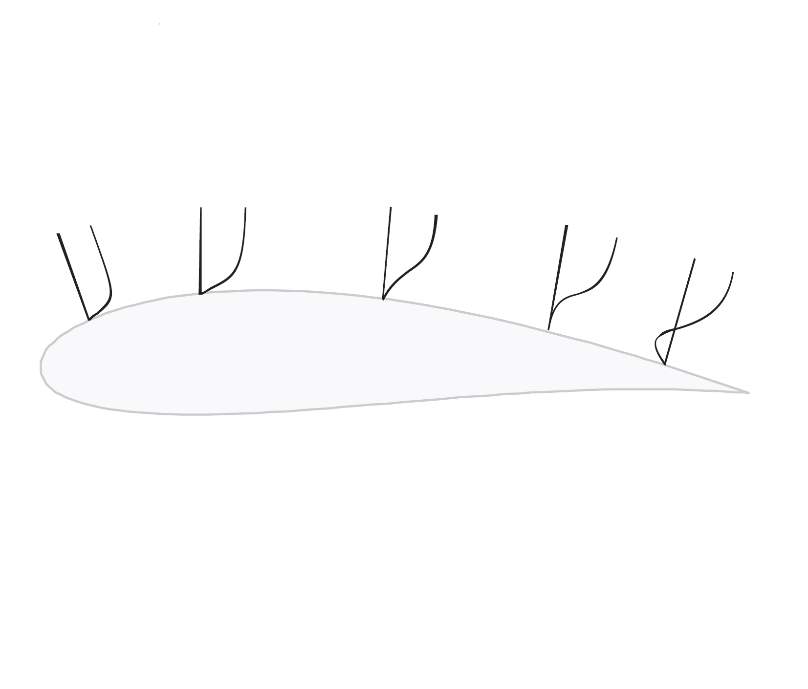
So, where should you start?  We have learnt that the wall function approach and y+ value required is determined by the flow behaviour and the turbulence model being used.  If you have an attached flow, then generally you can use a Wall Function approach, which means a larger initial y+ value, smaller overall mesh count and faster run times.  If you expect flow separation and the accurate prediction of the separation point will have an impact your result, such as the drag or lift forces experienced by the ellipse below, then you would be advised to resolve the boundary layer all the way to the wall with a finer mesh. Please refer to this post for a more detailed explanation of appropriate turbulent wall function and modelling approaches.

Wall Function applicability

Once we know our preferred approach, we can estimate the thickness for our first inflation layer cell using the equation below, which can be used to calculate the distance value for a specific velocity fluid and the required y+ value (based on the flow over a flat plate).  This is usually a good initial estimate and the y+ value we aim for will depend on our turbulence model selection.

\Delta y = L\cdot y^+ \cdot \sqrt{74} \cdot Re_L^{-13/14}

Note that Δy is the distance of the first node from the wall, L is the flow characteristic length scale, y+ is the desired y+ value, Re_L is the Reynolds Number based on your problem's characteristic length scale.

Unfortunately, as the y+ value is dependent on the local fluid velocity which varies across the wall significantly for most industrial flow applications, it is not possible to know your exact y+ prior to running an initial simulation.  For this reason, it is important that you get into the habit of checking your y+ values as part of your normal post-processing in ANSYS CFD-Post so that you can make sure you are in the valid range for your flow physics and turbulence model selection.

Our next post in this series concentrates on the feasibility and selection of different wall functions, based on the applied turbulence modelling strategy.

This is still an area of active research and is a hot topic for many of our CFD users.  If you have any questions or comments, please leave a message below or contact our CFD Technical Support team for more detailed technical information on these topics.

78 comments

  • I would like to ask a question about the range of non-dimensional distance y+. The range of y+ provided in this topis valid only for external flows or for both internal and external flows?...if so is true only for external flows then what will be the range of y+ for internal flows such as flow through pipes, non-circular ducts as we already know that internal flows become fully developed after a very short length of the duct which is oftenly neglected in basic fluid mechanics on the basis of assumptions. So, my point is that boundary layer in internal flows remain for a very short length of the duct and the flow become fully developed, so should we still adopt the same criteria of y+ for both type of flows, internal and external.

    • First of all, just to clarify your question, boundary layers will exist in the flow both before and after an internal flow becomes "developed". Developed simply means that the boundary layer thickness and velocity profile are no longer changing as we move along with the flow. So you will have a boundary layer at the start of a pipe (very thin), and it will increase in thickness until it reaches a steady thickness (developed). The thickness of this boundary layer, and how long it takes to develop, will depend on the Reynolds number of the flow, which is calculated from the pipe diameter, surface roughness, fluid velocity and fluid viscosity.

      You are correct that y+ is a non dimensional measurement of distance from a wall. It is used to describe the height of the first grid element next to a wall in a CFD simulation. We use y+ because experimental observation has confirmed that flows of all scales (big or small, fast or slow) tend to demonstrate very similar flow patterns as the flow approaches a wall. So Y+ is really used to identify where in the boundary layer profile our first calculation point resides. We can then utilise this Y+ number to determine the applicability of near wall turbulence modelling we intend to use, and these should be applicable regardless of internal or external flow conditions. So if we have a y+ ~ 1, we do not need any wall models and instead are resolving the flow all the way to the wall (typically with 10-15 cells within the boundary layer thickness as well as having a Y+~1). If we intend to use a coarser mesh and utilise wall functions to capture the near wall verlocity profile, we may aim for a y+ between 30 and 300. Whilst this range is often quoted as a general rule of thumb for both external and internal flows, it is very important to consider that the appropriate range of Y+ will vary according to Reynolds number also, and that higher Reynolds numbers (1e7+) will only accomodate a lower maximum y+ value (perhaps as low as 50 or 100). Beyond these values, the results will degrade and you will not be accurately capturing the near wall flow behaviour.

  • I am to use the k-omegaSST model for the 2D turbulent flat plate boundary layer flow and wish to compute u+ vs y+ curve at the point corresponding to Rex of 5x10^6. What are the Boundary conditions and initial conditions I should consider while running my simulation? Also that the flat plate starts some distance aft of the inflow plane. This region ahead of the flatplate is the slip-wall. What Boundary and initial conditions should I set for this slipwall?

    • Hopefully we have understood your question correctly. Firstly, your domain size should be defined such that there is sufficient distance upstream and downstream from your object of interest (flat plate) that the boundary conditions do not impact the results. A velocity (or mass flow) inlet can be used as the inlet condition, and a pressure outlet/opening can be used downstream. Taking L as the characteristic length of the plate, we'd advise you to place your inlet boundary at least 5L upstream of the plate leading edge. In a 2D simulation, the side faces will effectively use a symmetry face condition, as this behaves like a wall (no through flow) but does not enforce a V=0 condition at the wall (FLUENT 2D handles this automatically, CFX uses a psuedo-3D approach with 1 element thick domain). Initial conditions of a uniform flow field equivalent to the inlet speed should suffice for this case, as such a case will generally converge rapidly. Note it is worth considering if the Reynolds number at which you wish to measure the flow is fully turbulent, since by using the SST model you are assuming the flow is fully turbulent from the inlet. For transitional flows, greater accuracy will be obtained by using the SST model with transition, which not assume full turbulent flow but instead calculate additional equations which capture the transition of the boundary layer flow from laminar to turbulent.

  • Those were some very useful tips on wall y+ and near wall modeling. I'm facing a problem in choosing the correct near-wall distance in my pipe flow model. I'm estimating pressure drop in a low Reynolds number turbulent flow (Re ~ 10000) for a pipe diameter of 16 mm. I'm not sure which turbulent model I want to use: SST k-omega or a standard k-epsilon model. I know that for a k-epsilon model, I can get away with a coarse mesh and get my results quicker, but this means I can only fit in 3-4 inflation layer prisms (~3-4 mm) in my narrow 16 mm pipe so that my y+ values are in a suitable range.

    Is it always recommended to use an SST k-omega model if it becomes difficult to fit a larger number of inflation layers in a narrow zone? Wouldn't fewer layers mean more tetrahedral elements which affect the accuracy of my pressure drop calculation?

    • Thank you for your comment. The SST turbulence model has become the industry standard RANS model due to its superior accuracy in capturing flow behaviour in the near-wall regions. For boundary layers in adverse pressure gradients, to correctly predict flow separation it is imperative to have a Y+ less than or equal to 1, meaning we are resolving the boundary layer flow all the way to the laminar sub-layer. For this reason the low-Re SST model is ideal, since the use of the k-omega formulation for the boundary layer region means we can resolve to the viscous sub-layer and no extra wall functions are introduced. In the free-stream, the SST model switches to a k-epsilon formulation which is better suited to free shear flows. Therefore, we definitely advise the use of the SST model for your problem. For well-behaved wall bounded flows with mild pressure gradients, or for flows that are not dictated by boundary-layer effects, the k-epsilon model could comfortably be used.

      In regards to your question regarding the mesh, you are correct in saying that using the k-epsilon model allows you to can get away with a coarser mesh as you would be using wall functions to approximate the turbulent boundary layer profile. However, to resolve the flow down within the laminar sub-layer and gain a more accurate prediction of the velocity distribution and heat transfer in the near-wall region, we recommend the low-Re SST model which requires a finer mesh adjacent to the wall with a Y+ of 1 or lower and at least 10 prism layers within the boundary layer.

  • Hi, and thank you for this article which answers clearly to many questions.
    Nevertheless, there still are some remaining :
    When you study an external flow and that you expect a detachment of the Boundary layer, you tell that we should use a finer mesh near the wall to avoid using the wall laws.

    For my case, I use the k epsilon turbulence model.

    Is it possible to define some parts of the layer where we apply the wall functions and others - where there is detachment - and where we decide to not apply it, thus refining the mesh to compute in a finer way the boundary layer ?

    Thanks for all

    • Thank you for your post. If we idealise your problem as the ellipsoid as shown in our post, then you can imagine that the turbulent boundary layer will initially have a favourable pressure gradient (remaining attached). As the flow moves downstream and we pass the highest point of curvature we would expect to see the turbulent boundary layer at some point to move into an adverse pressure gradient, subsequently detaching from the surface as it approaches the trailing edge. In this case we have a boundary layer profile which is initially attached, inflected, and then separated and a pressure gradient which is constantly changing. For this reason we would strongly advise the use of a low-Re turbulence model (such as the SST model), which is able to resolve the boundary layer all the way to the laminar sub-layer. In a mild or zero pressure gradient, you can opt for a wall function modelling approach such as the k-epsilon turbulence model, and perhaps split your domain, whereby different domains may have different turbulence models. However this is quite tedious and unnecessary. In your case you could exploit the scalable wall functions feature in ANSYS. This means that different areas of the ellipsoid may have a mesh of varying density and Y+. The scalable wall functions will automatically activate the local usage of the log law in regions where the Y+ ~ 1, and standard wall functions in coarser Y+ regions.

      If you let us know what code you are using, we can give you some more specific information

  • I'm going to simulate an axisymmetric injector, by LES turbulence model, I would like to know as I'm using LES; and for LES, very small y+ is needed (y+ ~ 1), then using wall function is suitable or applicable? in other word can i use wall function to increase grid size near wall?

    Best Regards

    • Traditional LES models differ from RANS models in that the largest turbulent structures in the flow are resolved completely, while smaller structures (which can be argued have a negligible influence on most flows) are modelled using a subgrid-scale model. This makes LES inherently more computationally expensive than RANS models. In free shear flows, the turbulent scales are quite large so LES is suitable, however one of the most prohibitive limitations of LES is that within a turbulent boundary layer, the turbulent structures are quite small – and need to be resolved in both space and time. This means that the y-plus must be of the order of 1, and our cell aspect ratio in the boundary layer in both streamwise and crossflow directions should be of the order of 1 – 10. : Furthermore, since turbulence is inherently a 3D phenomenon, it is not suggested for 2D of axisymmetric applications so we recommend that you incorporate a 3D periodic slice of your injector instead.

      If you are interested in using LES for your simulation yet you would prefer to adopt a less conservative mesh for the boundary layer region we suggest the use of the Wall-modelled Large Eddy simulation (WMLES), Detached-Eddy simulation (DES) or Scale-Adaptive simulation (SAS). They all differ in their approach but inherently each method aims to resolve the large free shear turbulent structures using the LES technique and adopt a wall modelling or RANS approach to model the small structures in the turbulent boundary layer. Such models allow for more aggressive stretching of cells in the streamwise and crossflow directions (as per a RANS mesh) , yet it is our recommendation that you still aim for a y-plus value of 1.

    • I really like this post which is really very useful. I have few things into my mind which may be repeating the questions, apology for that.
      My questions are:
      1. What exactly meaning of "wall function" and what exactly happens in "Enhanced wall treatment" ?
      2. which parameter plays important role in turbulence modeling formula for wall function methodology?

    • Hi,

      The answer to these questions and any other concerns you may have with when and how to implement wall function is addressed in Part 3 of this blog series (Selection of wall functions and Y+ to best capture the Turbulent Boundary Layer)

  • Hi,

    Thanks for the great article. Finally it's something that gives a clear and concise description of y+ and answers a lot of my y+ and mesh inflation questions.

    However, I'm wondering if you could give some suggestions/advice for my specific application. I'm simulating the flow through a centrifugal slurry pump. For meshing along the boundary layer of the impeller especially as well as the volute, should I be using a wall function? It seems that I'm finding that a wall function would not be appropriate. It also seems that in the article above that for turbines, the Re is low enough that you suggest avoiding wall functions. In this case, should I be aiming for a y+ value of ~1 for the walls? In other words, should I be fully resolving the boundary layer?

    Thanks for your help and for all the good resources on this site!

    • Hi,

      Our suggestion here would be to use the SST turbulence model with curvature correction (this adds a production term useful for better predicting swirling flows). This will provide accurate wall-bounded effects in a centrifugal-type geometry with the added robustness of the two-equation SST turbulence model. Our suggestion is to aim for y+ value of 1 with sufficient prisms in order to capture the full growth/development of the turbulent boundary layer. Please refer to Part 4 (Reviewing how well you have resolved the Boundary Layer) for further details on post-processing the boundary layer.

  • Hello LEAP Support Team,

    Great article, really helpful. I followed your instructions and finally reduced my y+ from 10^4 order to below 300. I am modeling a 2D disinfection contactor (in drinking water treatment process) using realizable k-epsilon model with standard wall function.

    However, i have a very wide y+ range from 3 to 120. The small y+ can be found at a lot of different locations which makes it hard to re-mesh the "bad zones". And I also find adapting y+ seems not working for some reason. Every time I adapt the y+, set the minimum y+ value to 30, run calculation, the y+ profile doesn't change at all. Could you please help me solve this problem?

    Thank you very much!

    • Thanks for your question.

      The modern implementation of turbulence models in ANSYS CFD are y+ insensitive. This ensures that regardless of where our first grid height lies, we will be modelling the boundary layer profile comparatively. In regions where we have a low-Re type resolution, then we will be resolving the viscous sub-layer as well as the fully turbulent region. If we have a high-Re or wall function type resolution then we will modelling the fully turbulent profile. However, adopting a standard wall function approach in this case would give erroneous results in regions where we have low-Re type resolution, as the k-epsilon model performs poorly in this region. In this case you should resort to an appropriate low-Re model (i.e. SST) with the automatic wall treatment in ANSYS CFD whereby it will resolve the viscous sub-layer wherever applicable and then automatically default to a wall function approach on a relatively coarser mesh. If we want to ensure that we have a similar level of near-wall resolution everywhere in our domain (despite being constrained by varying scales of geometry – as in your case) then the scalable wall function offers a very elegant alternative. In this case you can continue to use the realizable k-epsilon model, however you can adopt the scalable wall function approach. When using this approach, the solver will virtually displace the wall-adjacent grid to ensure it will not attempt to resolve the laminar sub-layer and maintain consistency through the entire domain.

  • Thank you very much for your informative and knowledgeable post. I am really benefited from the post.

    I would like to know that the equation of flat plate you are mentioning here, what is the reference? Like book or journal actually derivation.

    Actually, mainly I would like to know the which expressions of skin friction coefficients is been used to derive the equation? As there are many expression of skin friction function for flat plate.

    Please let me know, I would be grateful to you.

  • Hi guys,

    Great blog, there is some really useful stuff on here! I have a question about the equation for determining the thickness of the first inflation layer. In the equation listed in this post, the square root is of 74, while in the ANSYS solver modelling guide it is the square root of 80. Is there any reason for the difference?

    Also, can you please confirm that this equation can be used for turbulent internal flow in pipes as well as external flow. If this is the case, am I right in assuming that the characteristic length is the pipe diameter for pipes?

    Thanks guys, much appreciated.

    Michael

    • Hi Michael, thanks for your question.

      The y+ value is simply the non-dimensional wall-adjacent grid height, which is a function of the fluid properties and the skin friction coefficient. For each geometry, when estimating the appropriate wall-adjacent grid height, there may be ambiguity in its correlation with our desired y+ value since the skin friction coefficient value is obtained from the calculated flow solution, and is not known in advance. In order to achieve an estimate, we are therefore required to use empirical correlations which are ultimately a function of the Reynolds number. Empirical correlations exist for both internal flows and external flows, and differ according to the baseline geometry and empirical functions utilized. We will be addressing this query directly with an upcoming blog post, giving a complete formulation of the procedure to estimate the wall-adjacent grid height.

  • Thank you for this article.

    The fourth paragraph states, "flows with very high Reynolds numbers ..., whereas low Reynolds number flows .... the use of wall functions for these class of flows should be avoided."

    To what class of flows does "these" refer? High-Re flows or low-Re flows?

    Thanks.

  • Hi and thank you for helpful tips! i have a question about y plus value and I hope that my problem is solved. i want to get aerodynamic coefficients for a hatchback car and i'm using wall functions. i use realizable ke with standard wall function and the average of y plus values for the body is 49. now i want to know: 1- is 30<yplus avg<300 a good range in my case?! 2- what wall function is better for my case? as regards i try to use non equilibrium wall function and the result is very close to standard wall function.

    thank you!

    • If you place your first point at of your inflation layer at 50 < y+ < 500 the flow in the viscous sublayer and buffer layer does not have to be resolved and wall functions are used instead to calculate these values. We would suggest to employ the SST omega model with automatic wall treatment in your case. The automatic wall treatment allows a consistent y+ insensitive mesh refinement from coarse grids, which do not resolve the viscous sublayer, to fine grids placing mesh points inside the viscous sublayer. Fortunately, for hatchback car aerodynamics the flow separation is highly likely to occur at abrupt changes in the car geometry (as intended by the designer) so acceptable accuracy can be achieved using a suitable wall function mesh.

  • Hi,Thanks for the great article
    I am analysing a ship hull and I am using k-e model.In mesh I want to know that my total boundry layer must be higher than the first tetra mesh or the tetra nods should cover boundry layer.
    thank you

    • The location of the first cell node should be chosen according to the approach you like to follow, that is if you want to use wall functions or resolve the BL. As reported by the Practical Guidelines for Ship CFD Application by the ITTC – Recommended Procedures and Guidelines. Wall functions are based on two-dimensional flow, typically at zero pressure gradient, and it is well known that the validity of these analytical expression becomes less, or even disappears, with increasing adverse pressure gradients. Thus it cannot be expected that the wall function approach leads to reliable and accurate solutions near a ship stern, where the flow is strongly three-dimensional and running up against an adverse pressure gradient. Thus, this is a trade-off between accuracy and computational effort that you must consider.

  • Dear LEAP Support Team
    I am simulating an internal flow inside a square cross section duct.the values of y+ differ up to 7.5
    as I know for viscous sublayer 5<y+<7. what do you suggest me?use a finer mesh or use the current mesh?
    thanks.

    • The laminar sub-layer actually exists in the range of y-plus < 5. Since you are dealing with an internal flow, which is more forgiving on the boundary layer resolution compared with external flows, we would be inclined to say that your resolution is sufficient for either the SST model or the k-epsilon model with scalable wall functions. Note that we do not have adequate knowledge of your problem to say this definitively. Obviously, if you have a surface where you are also expecting to resolve thermal gradients (i.e. conjugate heat transfer) then we would suggest further refinement to the recommended y-plus of 1 with an appropriate turbulence model for wall-bounded flows, such as the SST model.

  • Hi is SST k omega model and Transient SST model are same in FLUENT. How can I select SST k omega in FLUENT analysis. Pls reply me

    • Thanks for your question. We take it that you are referring to transition SST and not transient SST (which is a different topic). The SST k-omega and SST transition models are fundamentally the same, with the exception that the SST transition model solves for two more transport scalars, the turbulence intermittency and the momentum thickness Reynolds number. These two scalars are solved to quantify how turbulent the flow and is thus can be used to predict laminar to turbulent transition. This model is especially useful for external aerodynamic-type flows where the presence of the laminar boundary layer from the leading edge will affect the distribution of forces and flow patterns. The Reynolds number range where transition would have a large influence is 1e5 < Re < 1e6.

  • Dear LEAP Support Team

    Thank you for your decent website. It is really helpful and useful especially for those who are new in CFD to get the great tips and tricks. I hope you continue to write for us. I have a problem related to modelling floe in pipe. It would highly appreciable if you help me.
    I am trying to model turbulence flow inside a pipe with radios of 0.0762 meter and length of 5 meter at different velocity of flowing (6 m/s, 9 m/s, 12 m/s). I have been using K-e model (standard wall, Enhanced wall faction). I know I have get the Y+ < 5 for laminar sub layer. This requirement is fulfilled but during checking mesh ansys shows a warning of having high aspect ratio
    But it is really difficult to have y+ <5 and proper aspect ratio simultaneously. I have been trying different meshing actually I can get the better results in multizone mesh with body size of 0.007 and inflation of 20 layer and Max thickness of 0.001m with growth rate of 1.2. Could you please let me know how I can handle this? Is it proper to use SST instead of K-e regarding that Re number is about 39000. Please help me with detail explaining as I am new in CFD

    thank you for your time and concern

    • As you mentioned, it is sometimes difficult to obtain low-aspect ratio grids when performing simulations with high resolution grids near walls. However – we can ignore this warning message if the high aspect ratio cells area adjacent to no-slip walls. In the boundary layer, highly anisotropic grid sizes are permitted since the streamwise flow gradients from one adjacent cell to the next are negligible compared to the wall-normal gradients. To aid in convergence on meshes with high anisotropic cells it is useful to use the Coupled solver with pseudo-transient formulation

  • Thank you for your quick response. I have two question related to Y plus again.

    1- I am trying to have y+<5 while using K-epsilon method (enhanced wall) in a 5 m pipe. My y+ results give a value of less than 5 but the earlier values are about 8 and then it downs to less than 3 severely. Is this ok or not? Y plus value must be less than 5 throughout the geometry wall?

    2- My goal is to find pressure drop throughout a pipe. The amount of pressure drop changes with quality of mesh even for the Y plus value less than 5. For example when for the y+=3 I have dp=3600 Pa and for y+=0.5 I have dp=3400 Pa. which one is true?
    Thank you for your attention to my request

    • The reason for this is most likely due to the fact that your flow in the early stages of the domain is yet to achieve a fully developed profile. You can avoid this by specifying fully developed turbulent velocity, kinetic energy and dissipation profiles. For your second question, the sub-layer profile exists within the range of y-plus < 5 which suggests that the finer mesh resolution is expected to give you more resolution of the laminar sub-layer and therefore greater fidelity in your results.

    • how to calculate the value of turbulent vel , KE and dissipation rate of fully developed profile in a pipe flow

  • this is a very helpful blog!

    I'm simulating unsteady (transient) propagation of a pressure wave moving through a circular pipe. My question - is at the wave front the y+ value is ~ 52, while in the area behind the wave the y+ ~ 1, i'm guessing in this case I should only be concerned with the value of y+ at the wave front, is that a fair assumption ? or do i need to be more aware of how the y+ value changes?

    i've used the k-epsilon model initally and now i'm goning to try the sst model, hence my question as i would need to refine the mesh.

    thanks

    • Hi David, within a pipe your results will be less-dependent on resolution near the wall (as far as y-plus values) but we expect that you might find some discrepancy between different turbulence models. This is a perfect example of being able to use y-plus insensitivity which is the default treatment for the SST model, and is the scalable wall function for k-epsilon models.

  • I Have a Question and expect some support for you. According to the theory, depending upon the y+ values the flow region is categorized into different regions: y+ upto 5 is a viscous sub layer, from 30 to 200 it is log region etc. According to the theory the fluid velocities vary with different laws in different regions like viscous sub layer, log law region. Can you please suggest any paper in the literature or any such article which corroborates the claim with experimental evidence.

    • This is well documented, we suggest you start with the ANSYS documentation and refer to the appropriate section + the reference list that is found there.

  • hi LEAP Support Team i am working in simulating the flow and heat transfer in a ribbed rectangular duct using kw sst model for different Reynolds number , y plus less than 5 for all case , i want to compare results with ke RNG model , i want to ask if i should in my case to select the enhanced wall treatment in the RNG model or not ?
    (the mesh is equal spacing and adapted in wall regions )

    • Enhanced wall treatment should be the default treatment for epsilon-based models if you want to resolve all composite regions of the turbulent boundary layer. If you are solely interested in capturing the log-law then the scalable wall function should be utilized, as it will be virtually displacing the first cell height such that it neglects the sub-layer region.

  • thanks for your great blog.
    I'm simulating 3D steady flow over a heavy truck in fluent.It's almost impossible for me to reach y+~1 region because the solution becomes so heavy that i run out of RAM.(so i guess i'm going to use standard wall functions)
    my y+ is around 30-1000. i can adapt my mesh and bring it between 30 and 300. if i'm going to use k-w sst model do i need to have y+ in this range? and in general, in my case,which viscous model you suggest i use?
    thank you.

    • We recommend that you either increase your hardware capacity to improve your near-wall mesh, or if this is not possible then you can change to k-epsilon models with wall functions (realizable preferably.

  • Why and how prism layers resolves the boundary layer? Why can't we utilize tetra elements for the same. Thanks.

    • Prism layers are three dimensional mesh elements that are extruded from unstructured triangular surface mesh. They provide high-resolution of the boundary layer with multiple layers perpendicular to the wall (providing high fidelity for the near-wall Y+ and a slow transition/growth rate normal to the wall). The use of tetra elements to achieve the same goals would be highly inefficient, and tetrahedral elements cannot accommodate the high aspect ratios that prism elements allow without without sacrificing convergence stability and accuracy.
      In addition to prism elements, flow aligned hexa elements can be used to resolve boundary layers. ICEM CFD is an excellent tool for creating flow aligned hexa elements around complex shapes.

  • thank you very much for this course.
    is only the first row in grid has importance or the inflation growth rate and streamwise grid space is important too?

    • The first row is most critical (for Y+) but the inflation growth rate is also important to be kept to 10-20% max. Streamwise grid spacing needs to be used to adequately capture the curvature of the geometry, but you can tolerate much higher aspect ratios in the boundary layer (compared to the freestream) as the flow is aligned with the wall.

  • Hi. Thanks for the post!! is very helpfull!!
    I have a question. Is necessary to mesh with inflation layers exclusively???
    What happens if I succed in meshing with a mapped mesh and I achieved the desired y+ without the inflation layers.... Are the wall function working properly???
    Also, sometimes FLUENT gives me the warning that I have to check the "repair wall distance" even if I checked the y+ value... What does it mean??

    Thanks!!!!

    • Yes it is perfectly fine to have a mapped face mesh. Inflation layers are only required for hybrid tetrahedral topology grids. The wall functions do not factor the element type – only the height of the cell centre from the wall. The message that Fluent is issuing is related to high aspect ratio cells. Anisotropic grid spacing near the wall is acceptable provided streamwise gradients are negligible compared to the wall normal velocity gradients.

  • Hi, really great blog!

    I'm currently doing simulation of air diffuser (standard office/classroom) from 1-6 m/s inlet velocity and using realizable k-epsilon with enhanced wall treatment.

    my question is, how do we know our acceptable Y+ value? as i read from previous commends that they have already know their Y+ value and just need to compare with the Y+ value range after the Fluent process.

    second, do you have any recommendation for the solution solver setting?

    • Hi Aiman,

      Glad you are getting useful information from the blog.

      The acceptable Y+ range is a function of your modelling goals and resources available. After considering these factors, you should be able to decide if wall functions or boundary layer resolution is the best option.

      We can only calculate Y+ heights analytically for very simple shapes (flat plate, pipe, etc.). We can then use these approximations to give a first estimation of a first cell height for mesh generation. Of course, if you find that the resolution was insufficient when post-processing your simulation, it is a simple task to regenerate a mesh with finer boundary refinement and solve the model again.

  • Hi, thank you for your great information!
    I am using both k-epsilon and k-omega models fir my calculation.
    With k-epsilon, I use scable wall function and give nuce result compare with experiment. On the other hand, when I use SST k omega model, the results is different and I check y+ around 2-5. I read from some forum, they said SST model use enhanced wall but not exactly what y+ should be.
    Could you tell me about this problem?

    • Hi Le,
      The SST model can work equally well with a y-plus value of ~1 or of higher results in the log-law as it has automatic wall treatment, and is essentially y-plus insensitive for boundary layers in zero pressure gradients. Obviously for accurate prediction of wall-bounded quantities then it is in your best interest to resolve to a y+~1. In saying that - there is no universal RANS model which is applicable to all cases, and you should ultimately be doing your own turbulence model and mesh sensitivity studies when you have experimental data to determine the best modelling strategy. If you are getting better results with a k-epsilon model, then it is likely that the case you are looking at is not primarily dependent on wall-bounded flow but on other physics, perhaps mixing or shear layers?
      Regards,
      LEAP CFD Support

  • Hi,
    I use ANSYS Fluent for Room Air Flow Simulation studies. I usually have a 5x4x2.4 m box as my room and some openings as air inlet and outlet for supplying and exhausting air to and from the room. I use the inflation layer to refine the mesh near all walls surrounding my room but to tell the truth it's somewhat coarse (5cm thick and 5 layers). As the air flow path in the room is not internal flow in a pipe or air flow around an airfoil, I can not really judge how fine should my inflation layer be to avoid getting non reasonable results. Is there any criteria for y+ or infaltion layer for such applications?

    Thanks!

    • Typically for an application such as yours, the bulk flow behaviours are much more important than the wall bounded flow. In such cases, it can often be sufficient to have just a few inflation layers with the first cell height in the log-law layer (y+=20-200).

  • Anup Radhakrishnan

    Hi

    I want to simulate the flow around a 3D cylinder in turbulent flow and determine the characteristic coefficients like drag, pressure etc. I do not have adequate computing resources to resolve a mesh with y+=1 and hence would need to stick to wall functions. Please advise which wall function I should choose and an in what range the y+ should be adhering to.

    Thanks a lot for bringing up this amazing site.

    • If you are modelling the boundary layer with wall functions instead of resolving it with inflation layer, it is important that the first layer be in the log-law layer, which is y+=~20-200. If you use the recommended k-w SST turbulence model, the wall function will be applied for you. Do bear in mind that by using wall functions instead of resolving the boundary layer, your simulation will results will likely deviate from experimental or analytical values.

  • Hi
    Thank you very much, great work.
    I'm going to simulate incompressible oscillating turbulent flow through a pipe (D=50mm and L=5D) with pressure gradient that varies depending on the Womersley number at constant Re=1440. How can I estimate the y+?

    Thank you

    • With the varying conditions of your system, the best approach to determine the necessary first cell height will be to run a steady state solution at the maximum flow rate to determine the strictest boundary layer requirement. You can then proceed with the mesh accordingly.

  • Hi!

    Thank you for teaching us CFD in such a easy way! Your posts are really incredible, you become a reference for everybody who is beginning with CFD.

    I have a question for you: Can wall funcions be used for rotating walls?

    Thank you very much in advance!

    • Absolutely! Wall functions applicable to all walls, whether rotating, stationary, or with a specified velocity.

  • Hi I am trying to resolve a flow around a 2D circular cylinder and I am unable get the correct values for the Drag coefficients in the sub critical Reynolds Number region. I was wondering if this has anything to do with Y+ values around the cylinder wall/ i am using the k-omega SST model and and have gone to a really high mesh resolution and have still any achieved any substantial answer. My y+ values are now around 42 around the cylinder wall. What do you recommend?
    Thank you

  • Hi, I'm working on modelling hypersonic planes flying at low speeds (sharp edged geometries, resulting in lots of separation and vortices). After doing some reading I think the realisable k-epsilon model will be the correct model(?). I have currently have a mesh with a y+ ranging from 0.5 to 4.9. I am confused about which wall function I should use....If I further refine the inflation layer to ~1 is that better than using a wall function? Or is it better to leave the y+ and use enhanced wall treatment or a scalable wall function? I don't completely understand where each wall function is applicable...

    Cheers!

  • Dear LEAP support team, I am working on a 2-m long vertical thermosiphon and 2-cm diameter. At the bottom, I have a high temperature, at the top, ambient temperature. I guess that the water in the tube will have a turbulent flow. I want to measure the thickness of the condensated water layer at the top. I suppose I have to impose a y+ of 1 but how can I calculate the height of my first cell if I don’t know the fluid velocity? I may start from assuming the Reynolds number but I don’t know if it will be accurate. (I am still working as if it is single phase and I have not implemented multi phase yet)
    Thanks for your help!

    • True y+ values can never be known prior to solving. Even with the applet on this page, the values for cell height would be approximate. It is therefore normal and necessary to estimate, solve, review, and adjust as necessary.

  • Dear LEAP CFD Team,

    thanks a lot for your blog, it is always a pleasure read it.
    I am curious about transition from laminar to turbulent flow.

    Indeed I have a question about its identification and visualization. Is there any technique to extrapolate transition point from numerical simulations, or directly visualize it?

    On a flat plate I know that the calculation of the shape factor can give information about the flow state. But on bluff bodies, is such calculation meaningful? Or there are other variables which can be used to obtain this information?

    Thanks a lot for any help you can provide me.

    • If you are using a transition model you can gain insight into your flow field by investigating intermittency. If you are a current ANSYS customer, you can find the Guidelines for Laminar-Turbulent Transition Cases in ANSYS CFD document on the customer portal. This document discusses the various models available, model limitations, grid requirements, post processing, and more. You could also combine CFD results of a stable flow field with a stability analysis (again, considering the limitations of such analyses) to determine onset.

  • Dear LEAP CFD Team,

    Like the tips you have given above for various turbulence models, I am interested to know How can we prepare the mesh for LES/SAS model, means what should be the y+ values, how many layers should i put in the inflation layers etc.

  • Dear LEAP support team,
    I am simulating a convection flow in Ansys CFX using a quite complicated 3D hybrid mesh (tet + prism layers on the wall), which I generated in Ansys Meshing Tool.
    I have recently performed a Grid Convergence Study to quantify the spatial discretization error. The problem is that y+ continuously decreases when refining the mesh. At the end I got y+ lower than 5 for the fines grids and higher than 11 for the coarse grids.
    So, the boundary layer was resolved in the fines grids and modeled through the automatic wall function of the SST model in the coarse grids. That means that the error quantified in my grid convergence study corresponds not only to the spatial discretization error but also to the different wall treatment approaches used in the coarse and fine grids.
    Is there a method to separate quantitatively both errors when refining this hybrid mesh?
    When creating a grid which consists of only tet elements, won’t the boundary layer be resolved when refining the mesh? In this case, the error difference of the simulation results on the two mesh styles will correspond to the wall treatment error, isn’t it?
    Thanks for your help!

    • Typically when conducting grid Independence study you will want to keep the +y nearly the same to avoid the problem you stated. This can be achieved by keeping the first cell high constant and decreasing the growth rate and increasing the number of layers so the BL is correctly captured. Decreasing the growth rate will increase the number of cells for the same thickness levels.

  • Hi guys,

    Thank you for all these useful informations. My questions are the following:

    - How can I estimate the Boundary Layer thickness for a flow around an aircraft wing or fuselage for example ? Does using the Blasius solution based formulae give a sufficient indication ?
    - What is exactly a subgrid scale ?
    - What are scalable wall functions ?

    I will be very thankful for your answers.

  • Dear LEAP CFD TEAM,
    Thanks for your help,
    I am simulating a turbulent non newtonian fluid flow in annuli between two concentric cylinders, i am interested in predicting pressure losses, i am using a low reynolds k-epsilon model and i have some questions about it:
    1) i learned that the recommended y+ for this model is (y+<1), my y+ is 1<y+<2.5 for different fluid inlet velocities and results of pressure losses are close to the experimental ones with an error rounding between 0.5-21%. when i tried to get a lower y+ with reducing the first layer thickness, convergence became impossible what do you recommend to me?
    2) for a parametric study, in which i am changing the fluid inlet velocity the error increased with increasing velocity do i have to treat diferrently the near wall region every time i change my velocity, knowing that i have to use same number of elements in my simulations.
    3) How can i know that i am using the right parameters to treat accurately the flow boundary layer
    Thank you
    Regards

  • Y+ is a dimensionless quantity. That states what?
    Like the the region in viscous layer or log-law layer
    Or the height of the first cell?
    Please reply me as i am new to using cfd and this topic is really confusing me .

Leave a Reply to ali - Cancel Reply

Your email address will not be published. Required fields are marked *