
LEAP Australia has been working with university departments and engineering teams providing Ansys simulation software and technical support. The largest student engineering competition in Australia is Formula Student, where students learn how to design, build and race Formula 1 (F1) like cars around Winton Racetrack in Victoria. We actively sponsor university teams around Australia and New Zealand, providing licenses and technical support, giving us a unique insight into common questions posed by students.
Formula Student teams designing aerodynamics kits should understand the underlying physics, mathematical models and Computational Fluid Dynamics (CFD) concepts, which is difficult due to limited available public research. This blog post focuses on a common question: What y+ should I use in my simulations? To answer this question, the blog is broken into 3 parts in this series:
- Part 1 – Understanding the physics of boundary layers
- Part 2 – Resolving each region of the boundary layer
- Part 3 – Understanding impact of Y+ and number of prism layers on flow resolution
Part 1 – The underlying physics
What is the boundary layer?
The boundary layer refers to the fluid region near a wall where the viscous forces are significant, and for Formula Student, understanding how it behaves is necessary to determine how much force can be produced by a wing. An important aspect of the boundary layer is how resolving it helps predict flow separation. Flow separation on a front wing changes the amount of force it creates, and the flow field behind it, affecting cooling, the diffuser and rear wing. By understanding and controlling the boundary layer, engineers can maximise the effect of the front wing.
With a better understanding of the boundary layer, F1 engineers can control the flow from the front wing. Check out F1 engineer and Formula Student Aerodynamics judge Willem Toet as he explains how the front wing manages airflow around an F1 car in this video.
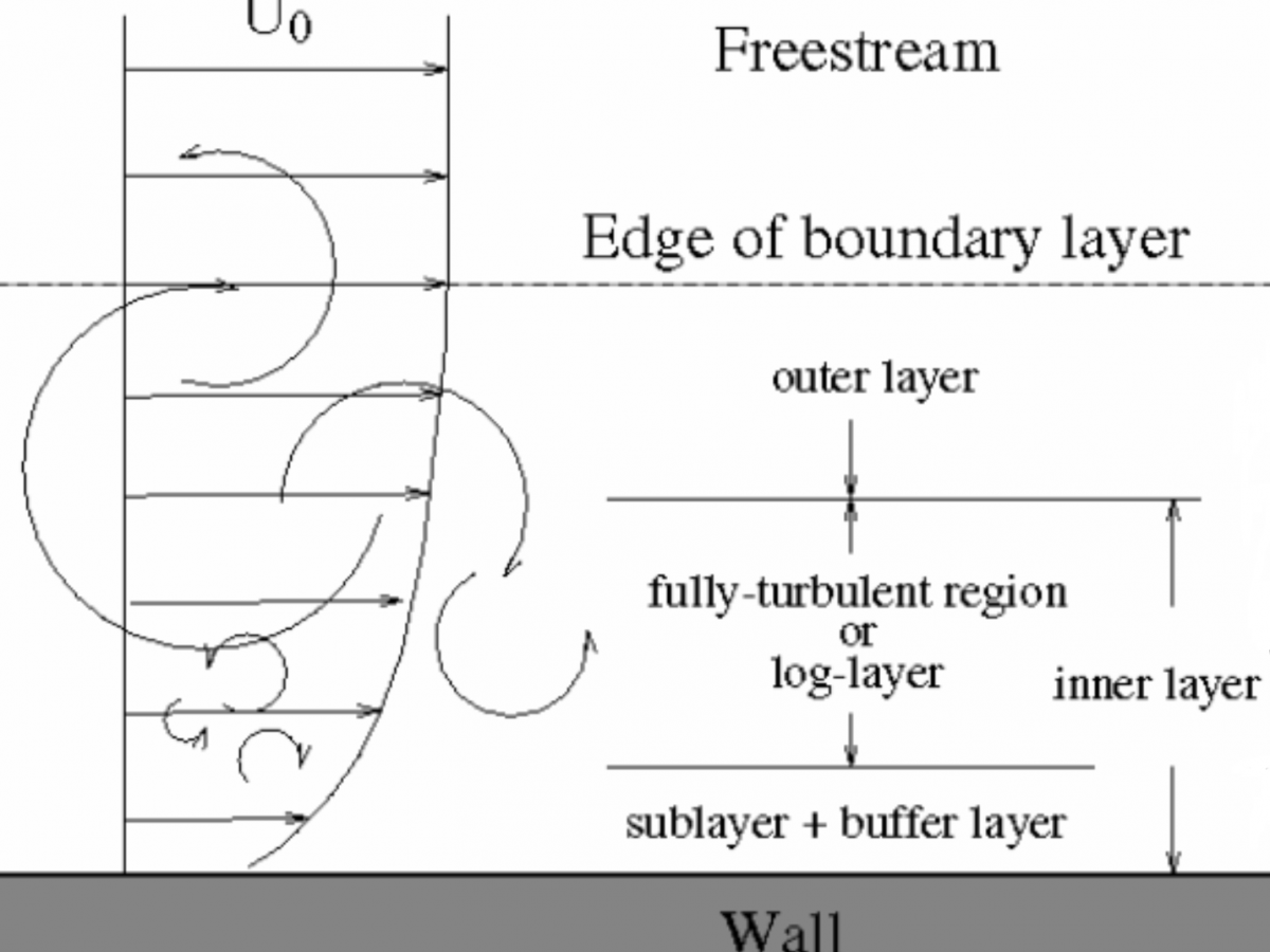
Now that we understand the importance of the boundary layer, let us look at its structure in detail. In the boundary layer, the velocity profile changes rapidly and can be broken up into three regions: viscous sublayer, log layer and outer layer, as shown in Figure 1 below.
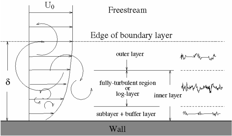
Figure 1 – Schematic of the velocity boundary layer (Source: Ansys Introduction training material)
Resolving the boundary layer close to the wall provides an accurate representation of its profile, leading to accurate predictions of wall shear stress, surface pressure, the effect of adverse pressure gradients and forces.
In FSAE, due to the shape of the wings, there are large pressure gradients that must be resolved to accurately predict downforce and drag.
For more information on boundary layers check out these videos: Click here
How does CFD resolve the boundary layer?
By using a log-scale and empirical equations to non-dimensionalise the velocity (u+) and the distance from the wall (y+), the velocity profile of the boundary layers takes on a predictable form, as shown below by the red line in Figure 2. There are two other equations, shown via blue lines, that have been derived capturing the profile of the viscous sublayer and the log-region. For more information about the mathematical equations check out here: Click Me (in this article u* and y* can be treated the same as u+ and y+).
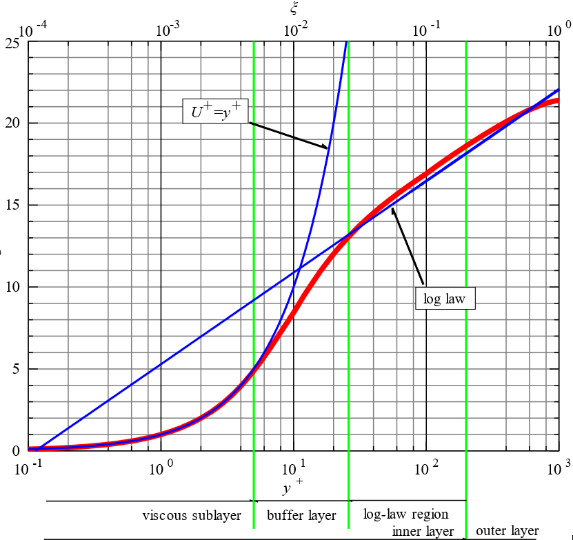
Figure 2 – Non-dimensional velocity versus distance from the wall (Source: https://en.wikipedia.org/wiki/Law_of_the_wall)
In CFD software the boundary layer is modelled by extruding the surface mesh elements at the wall. The surface mesh can be made up of different element types, but for the purposes of this discussion, we will consider triangular surface elements which are extruded into prism cells. The boundary layer resolution depends on the first cell height and the number of prism layers. The solver calculates a value, y+, which is computed from the first cell height, local flow speed and fluid properties. For the same fluid and flow conditions, we can say that reducing the first prism height by a factor of 2 will reduce y+ by a factor of 2. Obtaining an initial value for y+ and then adjusting the prism heights in the meshing tool or via adaption is a common practice in CFD when tuning the mesh for best results.
Different turbulence models are used to capture the boundary layer in different ways. The k-ω SST model has been widely researched, tested and is accepted as a good choice for many industrial problems, and has the robustness to resolve the viscous sublayer or the log layer. If the first cell height is in the viscous layer, it will resolve the boundary layer by evaluating the velocity at each cell. If the first cell is in the log layer, the software will make an empirical assumption about the viscous sublayer, referred to as using a wall function.
A careful selection of how you would like to model the boundary layer is essential.
When resolving the viscous sublayer, a value for y+~1 is required, which will require significantly more mesh elements and effort, Figure 3, left-hand image. This will lead to higher meshing and solution times and the requirement for more computer system resources. If you determine, that is not important to resolve the viscous sublayer, i.e. to use a wall function, a value for y+ > 30 is valid; this will result in less meshing effort and computational time, Figure 3, right-hand image. Note, however, that using wall functions can result in modelling errors, the significance of which will vary depending on flow conditions.
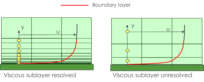
Figure 3 – Left – Near wall mesh when resolving the viscous sublayer, Right – Near wall mesh when using wall functions
(Source: Ansys Introduction training material)
It is recommended to either resolve the viscous sublayer by creating a mesh with y+~1 or to use the wall function approach by having the first element in the log region (y+ >30) and avoid having a y+ between those values. The models in Ansys CFD can manage the entire regime; however, it is good practice to make the intention clear and use one approach or the other.
The truth is most Formula Student teams do not have the computational resources to run a y+~1 for every 3D simulation of every design across the different yaw, pitch and roll conditions they desire.
With a better understanding of the boundary layer, how it is modelled in CFD and what y+ is, we can now address the question “Which one should we pick, and how many inflation layers are needed?”
Stay tuned for the next in this 3-part blog series:


