
The Australian government has outlined plans for significant investments in major infrastructure and smart technology projects in the coming decade to modernize the transport network in all major cities. As an example, in Melbourne, in addition to the Melbourne Metro tunnel, there are evolving plans for the addition of a suburban rail loop around Melbourne which will require significant tunnelling through built-up areas. This investment is critical in maintaining a reliable mode of transport that will be key to maintaining Australia’s liveability and prosperity as the population grows rapidly and the economy changes in the coming decades.
Train tunnels are common features of any rail network and often present some of most challenging problems for designers to solve when developing a new railway network. For example, the Metro tunnel being built in Melbourne to free up space in the city loop which will allow more trains to run in and out of the city.
Adequate ventilation is a critical component of designing a railroad tunnel. Fans are installed throughout the tunnel for ventilation and smoke control along the length of the tunnels. It is important to accurately size the fans to ensure that these fans perform reliably in scenarios when trains pass through the tunnels at high speeds.
Traditionally, 1-D or 2-D simulations were used to guestimate the average pressure inside the tunnel when a train passes through it. However, these simulations are unable to provide an accurate estimate of the velocity components, their magnitude and distribution, which is critical for accurate fan sizing. Designing a ventilation system for tunnels longer than 2 km calls for transient 3-D simulations to capture the evolution of the air velocities in the tunnel as the train goes through the tunnel.
COMPUTATIONAL SETUP
The computational domain is created using the following approach.
Extrudable volumes are created upstream and downstream of the train during geometry modelling in ANSYS SpaceClaim as shown in Figure 1 and Figure 2. Using this approach creates cells aft of the train and delete cells ahead of it as the train moves through the tunnel during the transient simulation. Inflation layers are created adjacent to the walls of the train to capture boundary layer effects in the simulation. The enclosure around the train is filled with tetrahedral elements while the rest of the domain has prismatic elements generated using the sweep method in Ansys Meshing. A non-conformal interface placed at the tunnel wall allows the train to move from one end of the tunnel to the other. The mesh quality is checked to ensure minimum orthogonal quality is greater than 0.1 before proceeding to the solver-setup stage of the process. An animation of the mesh evolution due to train motion is shown in Figure 3.
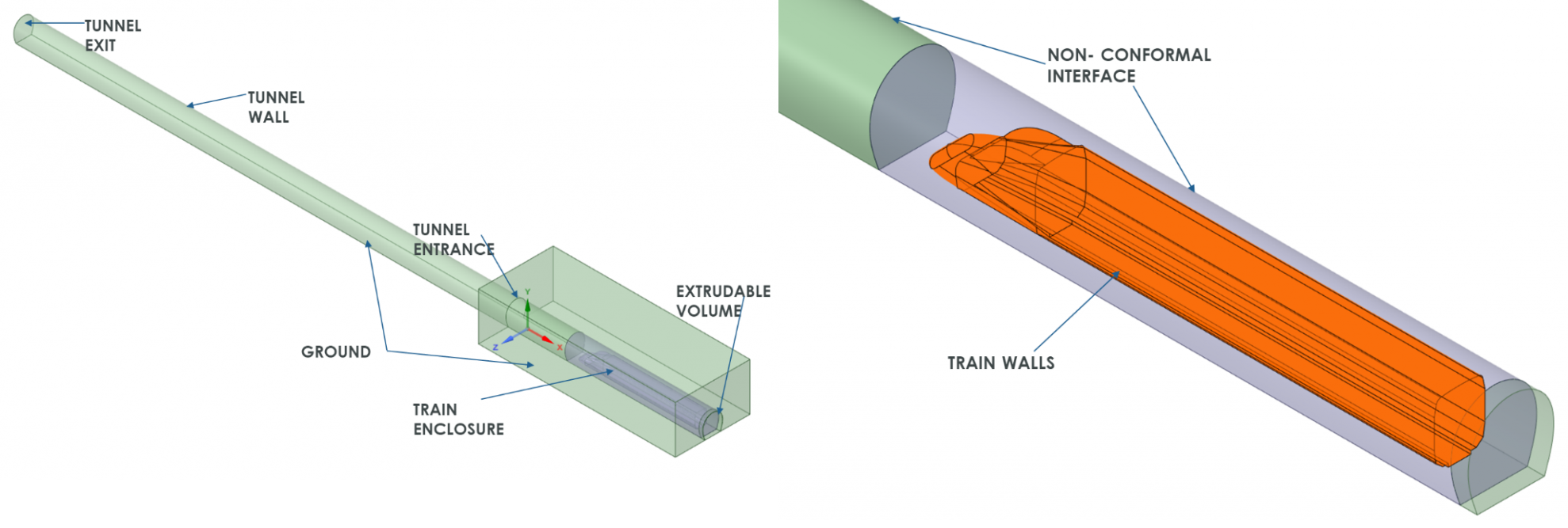
Figures 1 & 2: Computational domain in SpaceClaim Direct Modeler
Figure 3 Mesh evolution as train moves in tunnel
In this scenario, the train is assumed to start from rest and accelerate linearly with time till it reaches a peak velocity of 72km/hr in 20s. Due to the speed of the train, air is assumed to be incompressible with constant density. Trains travelling at speeds in excess of 200km/hr would need to account for the compressibility of air using the ideal gas law. Effects of turbulence is modelled using the industry-standard k-w SST model. The dynamic mesh zones are defined to ensure the cells are created and destroyed accurately in line with the motion of the train. The inlet to the domain is defined as a pressure inlet and the exit of the tunnel is set as a pressure outlet. Pressure based transient solver is used to perform the calculations and a time-step of 0.0005s is chosen to ensure solution stability. The Non-Iterative Time Advancement (NITA) scheme is used to accelerate solution convergence. The case and data files are saved every 0.1s and the results are post-processed in Ensight.
POST PROCESSING
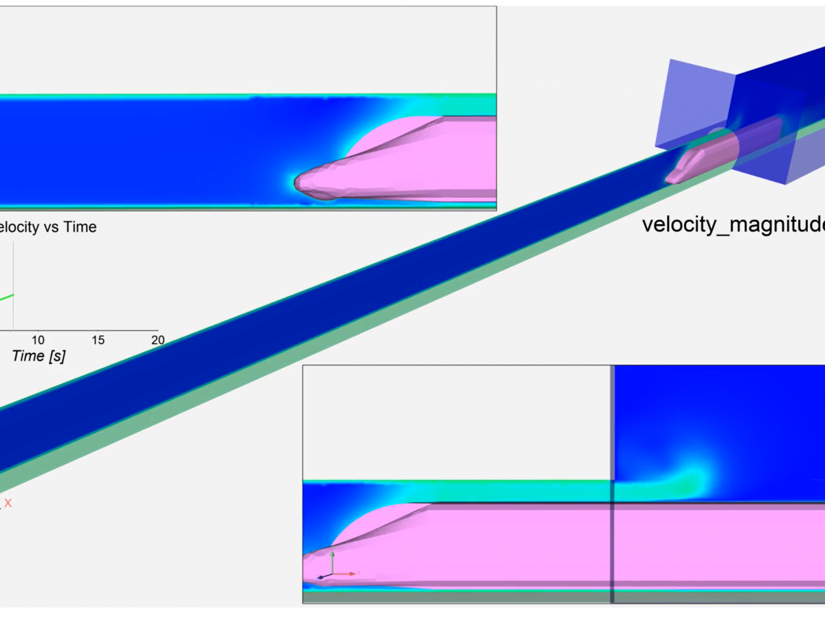
The flow patterns were analysed by plotting velocity contours at various sections of the tunnel. The maximum and minimum values of longitudinal velocities at these sections are plotted as a function of time. The evolution of pressure along the length of the tunnel is visualized by plotting contours of pressure at the symmetry plane. These contours provide insights into the complex flow patterns that are generated by the train passing through the tunnel.
When the train enters the tunnel, air escapes at the tunnel entrance through the gap between the tunnel and the train, mainly because it is the closest exit and because the air at the tunnel exit is yet to be put in motion. As the train goes deeper into the tunnel, air pushed by the train travels backwards in the gap between the train and the tunnel and creates the longitudinal air motion in the tunnel. Wind speeds up to 86km/hr were measured at the cross-sections as the train passed through them. Accurate prediction of these wind speeds is necessary to select the correct type of fans that can withstand these wind gusts and perform reliably.
Figure 4 Evolution of longitudinal velocities within tunnel
In addition to velocity variations mentioned above, the passage of the train creates significant pressure changes within the tunnel. Animation in Figure 5 shows the evolution of the pressure wave as the train moves through the tunnel. The train entering the tunnel acts as a piston that creates a positive amplitude wave that propagates along the length of the tunnel. When this wave reaches the end of the tunnel, it creates a booming sound that can be disturbing to local population and wildlife. The highest pressure seen in the compression front in Figure 6 corresponds to the time when the compressive wave reaches the end of the tunnel and creates the boom. CFD simulations can predict the amplitude of the pressure wave and this information can be used as inputs to an ANSYS Mechanical simulation to evaluate the effect of this boom on the walls of tunnel. In order to mitigate the tunnel boom, the bore of the tunnel entrance is extended and perforated with holes which helps to reduce the amplitude of the pressure wave.
Figure 5 Evolution of Pressure within the tunnel
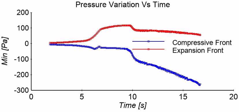
Figure 6 Pressure variation in tunnel vs time
The aft end of the train creates a negative amplitude or a compression wave in the aft of the tunnel. This causes air to get sucked into the tunnel inlet. The combination of pressure wave and compressive front cause noticeable accelerations and decelerations in the airflow within the tunnel. These complex flow phenomena are seen to continue even after the train exits the tunnel. These flow disturbances are not restricted to the longitudinal directions but also travel in the transverse directions. The main advantage of conducting a 3-D CFD simulation is that it can capture the transversal velocity profiles which can be of the same order of magnitude as the velocities in the longitudinal directions. Figure 7 shows the evolution of transverse velocities within the tunnel due to the motion of the train.
Figure 7 Evolution of transverse velocities within tunnel
This post has shown how high-fidelity 3D computational fluid dynamics simulations can provide tunnel design engineers with insights and a wealth of data on the complex flow physics arising due to the motion of trains entering and leaving a tunnel. This information can be used to refine the design of rail tunnels to allow faster moving trains without disruption to local residents and the environment.
For more information on Ansys CFD solutions, please contact your local LEAP experts across Australia and New Zealand.


