
Introduction
Engineers at LEAP work daily to support and provide advice to a mix of OEMs, engineering consultants and all the major universities around Australia and New Zealand. Our CFD support engineers work systematically with our customers to help troubleshoot any simulations that are not behaving as expected – and here we felt it would be helpful to document this ‘mental checklist’ which we often use to tackle challenging problems (in the hope that it will help you, also!).
You can learn more about the experience of LEAP's CFD team here. This checklist will focus on the Ansys Fluent CFD solver, however, we often start by reviewing the geometry and mesh. If you are also interested in seeing a “geometry and meshing” tips and tricks checklist, please let us know in the comments.
Naturally, when you start the troubleshooting process, you may already have a suspicion about the cause of your issue - so you may find yourself checking a few parameters, making multiple changes and then re-running/reviewing results. However, our first piece of advice is that, in order to identify the root cause of the problem, aim to make one deliberate change at a time.
To keep it simple, this blog is going to focus on steady-state, external flow, RANS simulations, however, this troubleshooting checklist is also a useful place to start for other flow types. We will focus on the following sections:
- Common problems; common issues causing the simulations to not converge
- Isolating the problem; isolate the problem areas
- Changing the solver; different variables you can use to tune your model
Common Problems
This section covers common problems when simulations don't converge
- Before starting your simulation have a solid understanding about the intended output and goal of your overall project. This will help you set up appropriate inputs, and sanity check your results when your gut tells you there is something wrong.
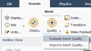
- Check mesh quality, which can be found under Domain, in the Ribbon toolbar.
- The results will be displayed in the console at the bottom of the window. Ensure Minimum Orthogonal Quality is above 1.0e-1, particularly for models of higher complexity, such as high-speed flow, heat and mass transfer and multiphase flow.

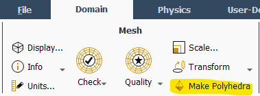
- If the Minimum Orthogonal Quality is below 0.1 and you have a tetrahedral mesh, try converting the grid to polyhedral.
- In the Domain tab, you can also improve the mesh
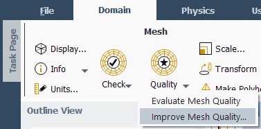
- This allows you to specify the percentage of cells to improve, and the number of mesh improvement iterations
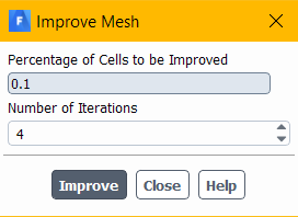
- The console will indicate how many cells were improved

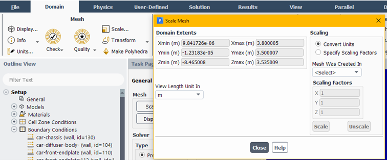
- Check that the units and scale are appropriate when compared with the physical geometry.
- In the Domain tab, Scale shows the domain extents with scaling options available on the right.
- Check the physics models you have selected and ensure they are appropriate for what you want to simulate.
- If the simulation has trouble converging, reduce the complexity and build it back up. This could mean solving laminar flow, before adding turbulence or applying a constant velocity inlet instead of a profile.
- Check boundary conditions and units, a common problem is misreading units, i.e. applying mm/s instead of m/s or applying incorrect direction vectors on rotating walls.
- If the boundary conditions you are applying are supplied from a physical test, ensure the location lines up with the physical test, and the appropriate flow conditions have been supplied. A common problem is specifying a constant velocity inlet with default turbulence conditions of a wind tunnel when in-reality a velocity and turbulent kinetic energy profile may be required.
- Is gravity required? If so, remember to check its direction, values and units
Isolating the Problem
With the common problems checked, the following section will provide tips and tricks to isolate the problem areas. In most situations, the flow field is complex with flow features from different components interacting. Identify which component is causing the issue is the next step.
- When the solution is running, check to make sure that forces and residuals are steady. Ideally, both monitor points and residuals should flatline
- If residuals and forces are oscillating around a mean, it may indicate inherent transient behaviour, and the pseudo-time step is too large. You can run transient for a few time steps or change the pseudo-time step, these points will be expanded in the next section.
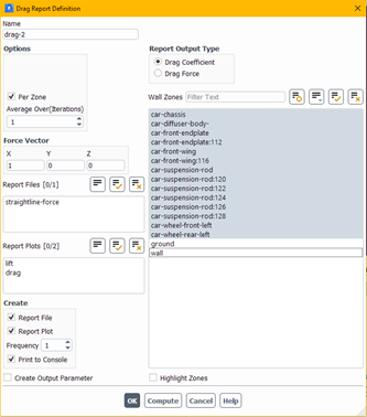
- Create monitor points to measure quantities of interest.
- As an example, if you have a race car with multiple components (chassis, wheels, wings), create downforce monitors on all the components and individual components. Understanding how the system and its components are behaving will help isolate which component is giving you trouble.
- Check the relevant contours and boundary conditions in post-processing.
- Use post-processing to double-check your boundary conditions, ie. Mass flow rate at inlets and directions vectors on walls
- Create cut planes to analyse the flow keeping an eye out for abnormalities in flow speed or direction.
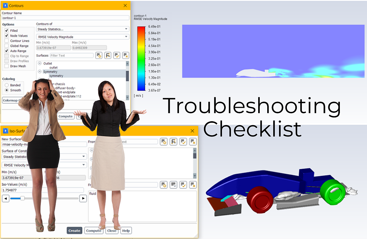
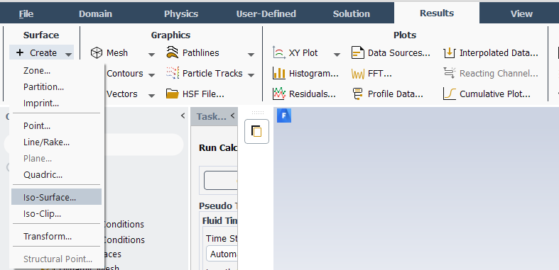
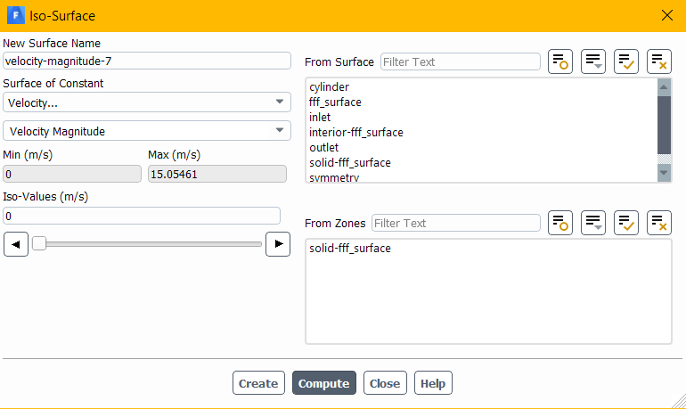
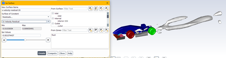
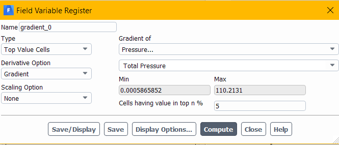
- Isosurfaces are an underutilised tool to identify abnormalities. Create an isosurface of low-quality mesh elements and others showing abnormalities like high velocities or pressures. If the overlapped isosurfaces align, you have identified the mesh regions that require fixing.
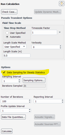
- Data sampling for steady statistics can be implemented showing where variables are fluctuating
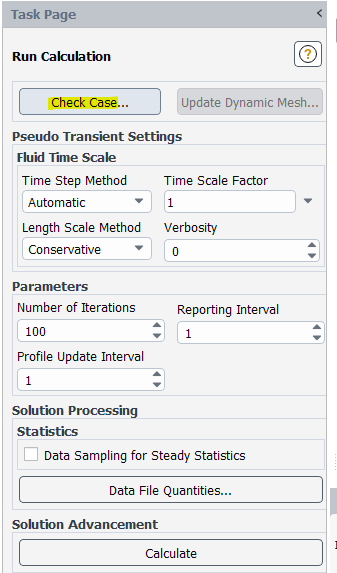
- Data sampling will sample flow variables over a specified number of iterations after it is turned on. It can be activated in the Run Calculation section - Activate data sampling for steady statistics
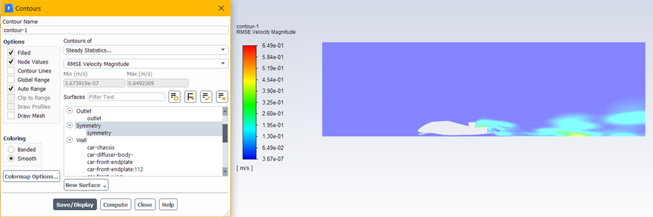
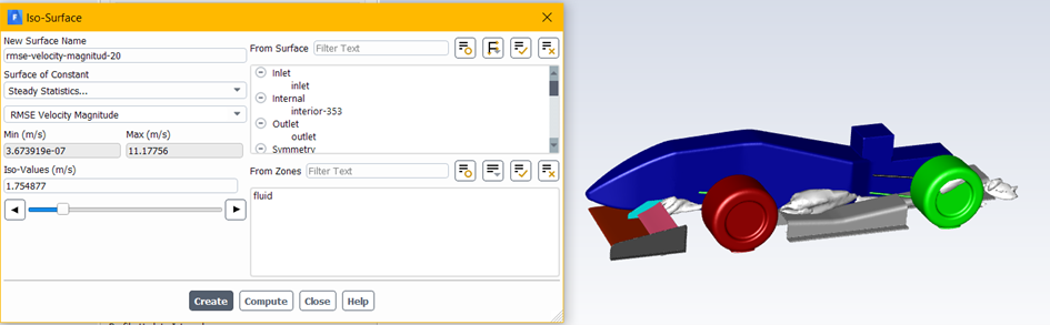
- After running some iterations, you can post-process the results in the new contour under Steady Statistics. Create contours or isosurfaces to view the mean quantities, or the root mean square (RMSE). The RMSE helps you identify where variables are fluctuating.
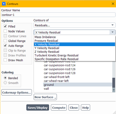
- To plot the residuals as contours or isosurfaces, write the following into the Console. This will save more data per timestep, taking longer to solve, so use only for debugging
- solve set expert yes yes yes
- solve iterate 1
- In the contour panel, you will be able to see more residual contours or create isosurfaces to depict where the residuals are high
- Generally, you will see high residuals around regions that have high-pressure gradients and where there are large jumps between cell sizes.
- Animation of variables is another method to visualise where the flow is fluctuating as the solver is iterating.
- Initialise the model and let it run. When your monitors start to oscillate, create a contour, isosurface or XY plots
- Wall shear on the component if the flow is separating
- Velocity on planes
- Turbulence Kinetic Energy in the wake
- Pressure plots on the surfaces
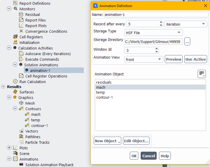
- Create a solution animation.
- Recording at every timestep will slow down the simulation, so consider writing them every 10 iterations.
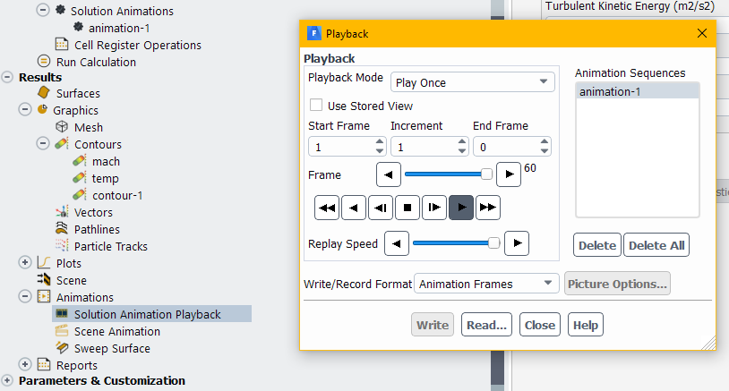
- Play the video back using the Solution animation Playback.
- Initialise the model and let it run. When your monitors start to oscillate, create a contour, isosurface or XY plots
Reviewing Solver Settings
After you have identified what variables are oscillating and where next comes changing the solver settings. There are different variables you can tune to help your model, there is no silver bullet and often comes down to trial and error. Make sure to change one variable at a time, saving case and data, if something goes wrong, you can always backtrack.
- In the Run Calculation window, the Check Case will provide some recommendations to help identify the potential problems
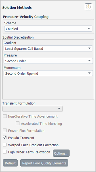
- Poor quality meshes containing highly skewed cells, highly non-orthogonal cells, non-convex cells, or cells with left-handed faces. Such mesh elements tend to decrease the numerical stability of the solver. By default, Fluent will apply 1st order correction scheme to these cells. A TUI warning will be displayed in the console, with a Report Poor Quality Elements button present in the Solution Method
- It is highly recommended to go back to the meshing process and fix these poor quality elements or use Fluent's mesh improvement tool.
- The mesh can be too coarse to resolve flow features.
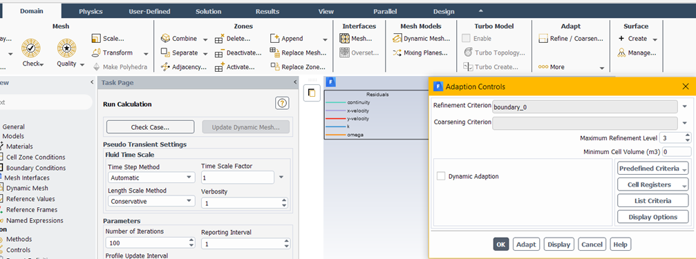
- Mesh adaption is available in Fluent, you can scope the physical region or variables for adaption. Fluent also has automatic mesh adaption for multiphase problems using the Volume of Fluid (VOF) model, which can dynamically refine the mesh in the required regions as the solution proceeds.
- A good initial guess can help converge a simulation quicker
- Use a hybrid or FMG initialisation to give your simulation a good initial guess
- The FMG initialisation can be activated using the Text User Interface
- /solve/initialize/fmg-initialization/yes
- More information can be found in the:
- If you continue to have issues at the start of your simulation, start the solver using first-order numeric, then switch over to second order
- Change the Relaxation factors
- Relaxation factors of equations are used to control the update of computed variables at each iteration. In Fluent, the default under-relaxation parameters for all variables are set to values that are near-optimal for the largest possible number of cases. These values are suitable for many problems, but for some particularly nonlinear problems (for example, some turbulent flows or high-Rayleigh-number natural-convection problems) it is prudent to reduce the under-relaxation factors initially. It is good practice to begin a calculation using the default under-relaxation factors. If the residuals continue to increase, you should reduce the under-relaxation factors.
- They can be changed in Solution>Methods
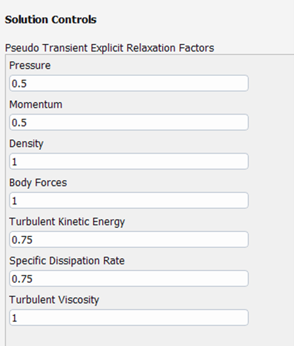
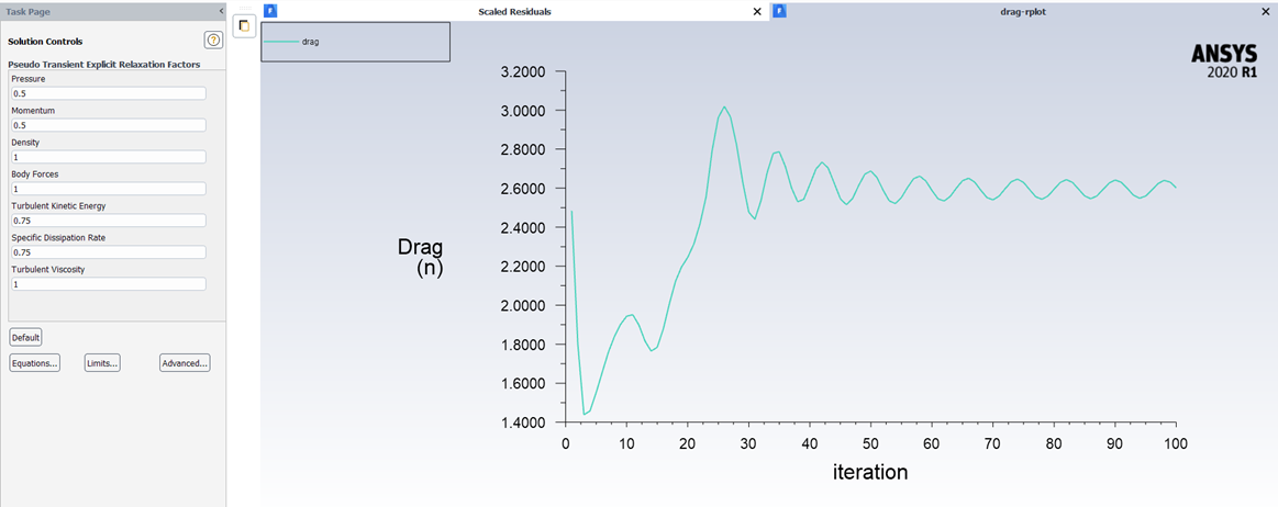
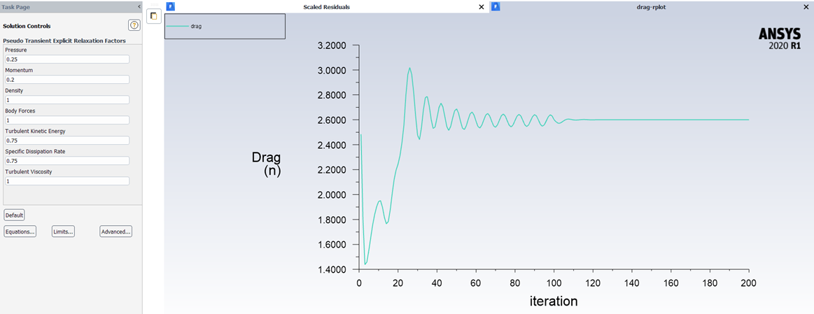
- The example below consists of flow around a cylinder. The first picture ran to 100 iterations with default Relaxation Factors, showing oscillating force monitors. Reducing the Relaxation Factors allowed the force monitors to converge after another 100 iterations.
- For your problem, reduce the Relaxation Factors by 10%, run the solution and observe the residuals and monitor points.
- More information can be found in the
- Change the pseudo transient time scale
- The pseudo-transient time scale is used in a steady-state simulation, it implements a timestepping-like approach to help with convergence. A large time step can accelerate convergence but may not resolve small flow features, leading to oscillatory residuals. A smaller time step can resolve small flow features but will take longer to converge.
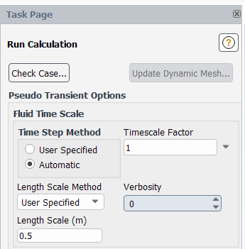
- The automatic timescale uses flow variables and domain dimensions to determine the pseudo time step
- It can be viewed by changing Verbosity to 1
- You can use the timescale factor to either increase or reduce it
- Another alternative is to implement a length scale based on the smallest feature the mesh is resolving. Instead of the solver taking the domain size, it will use the specified length scale to calculate the pseudo time step.
- You can then use the timescale factor to either reduce the timestep as required
- Another alternative is to estimate a pseudo-time step and use it directly in the solver
- A general rule of thumb is taking the 0.3*characteristic length/flow velocity. Characteristic length could be the length of the chord or internal diameter of a pipe. This is the preferred approach.
- More information can be found in the
- Flow is inherently transient, and the solver may be unable to calculate a steady-state solution. After running steady-state, switch the solver to transient mode.
- Run for a small number of timesteps. A good indicator of transient physical behaviour is an immediate drop in residuals when compared with those from the steady-state run. If residuals fail to reduce in transient mode, it is more likely that the model or mesh need adjustment. It is a good idea to take transient statistics if you would like to average variables over time.
With the above solutions, it is important to make one change at a time and understand how it affects the flow field before making more changes.
Summary
Hopefully, you can implement the checklist above when you have problems converging, or your results do not make sense. Some key elements to take away from this blog are:
- Make one change at a time when diagnosing a problem
- Common problems typically include mesh quality, scale, units and boundary conditions.
- Use monitor points when solving to make sure that the quantity you are interested in is converged, as often the residuals alone cannot determine if all solution outputs are converged. When things start to diverge, or the results are not steady, inspect the global and local quantities and post-process the results to identify the problem.
- Depending on the problem, make a change to your solver and review the results. Save case and data before making any changes, that way if something goes wrong you can always go back.


