
Guest Blog by Edward Yap, CFD Consultant and Deepak Jagannatha, Lead CFD Consultant at Wood Australia. Edward and Deepak recently presented this in-depth look at their analysis of a Subsea Christmas Tree as part of LEAP’s Ansys CFD Virtual User Group meeting.
Wood Australia is a global leader in consulting and engineering across the energy and built environment sector, operating in over 60 countries. The business itself is split into three main groups; consulting, projects and operations with the CFD department falling under the consulting group but also providing assistance to all sectors of the business as required.

Wood have 10 to 12 members globally that work full time on a range of different CFD projects in a range of different industries such as oil and gas, mining, renewables and even government organizations. The CFD group works on problems ranging from equipment designs, mixing and chemistry, thermal analysis, sand transport and erosion, vibration, gas dispersion and explosion and a range of many others.
During this user group presentation, Edward and Deepak discussed a recent CFD project undertaken by Wood Australia on a Subsea Christmas Tree, commonly used in the Oil and Gas industry.
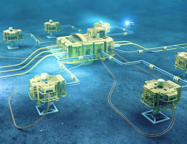
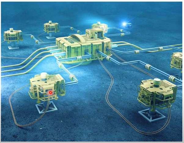
The image above shows a typical subsea configuration of ‘trees’ which are a complex assembly of valves and ancillary equipment which get installed at the top of the wellhead to control the production of hydrocarbons. Immediately downstream of these trees is a choke valve that allows the rate of the production to be controlled which then connects to a jumper line and multiple of these jumper lines then connect to a central manifold which then sends the production fluids to topside facilities or onshore facilities depending on where the system is installed.
One of the major concerns of offshore oil and gas production is the formation of hydrates which are essentially crystalline formed solids consisting of water and trapped gas molecules that form at low temperature, high pressure environments; which are very typical of shut-in conditions when fluids are left to cool to ambient sea water temperatures. To mitigate the formation of hydrates they are typically prevented through two main methods - one can be active hydrate inhibition which is essentially injecting fluids such as meg (monoethylene glycol) or methanol which shifts the hydrate formation point, or passive hydrate inhibition methods - such as insulation which retains that fluid temperature and leaves it above that hydrate formation temperature for sufficient time before intervention can occur.
This case study specifically looks at conjugate heat transfer simulations on a Subsea Christmas Tree. We are looking at both steady state and transient simulations using inputs from flow assurance discipline and the results of our simulation provide a detailed temperature distribution of these Christmas Trees to help us determine the amount of insulation required to achieve a three hour cool down time. A cool down time is defined as the time after shutting for a fluid temperature to drop below the hydrate formation temperature.
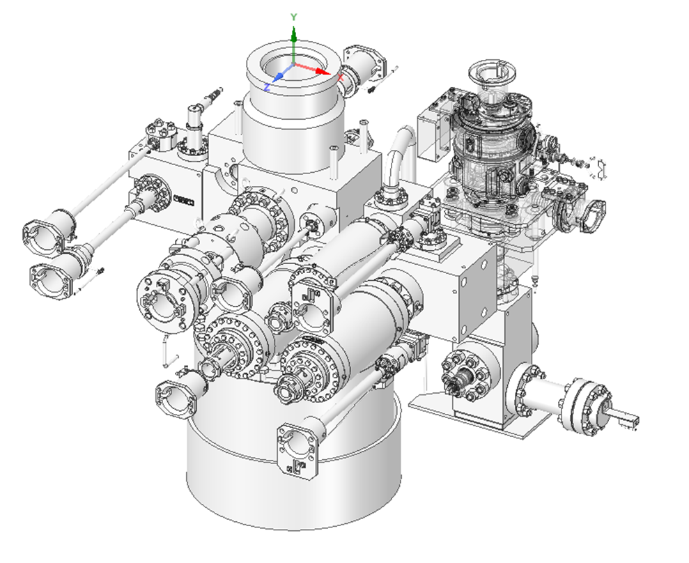
The picture above shows the original CAD geometry of a Subsea Christmas Tree that we were provided by a client. As you can see it's incredibly complex and there are many different parts. This specific one contained over seven thousand parts and it has also had a range of the structures removed so you are able to see the main Christmas Tree there. Clearly for us to run a CFD model on this involves a lot of CAD clean-up, which was done using Ansys SpaceClaim.

The image above shows the final cleaned up CFD model. As you can see, all of the supporting structures were removed as they are not required for the conjugate heat transfer assessment. The choke valve actuator has also been taken off and the piece that has been added is the jumper. This is mostly to capture the correct outlet boundary condition. You can also see that a lot of the shapes have been simplified however an engineering judgment has been made so that we are maintaining the overall shape and volume so that the heat transfer through the bodies is simulated correctly. Other things like small gaps and edges have been smoothed out or filled just to make sure that we're able to fit a high quality mesh into this domain.
The next image shows a cross-section comparison between the original CAD geometry and the final CFD model that was built. The original CAD model that we were provided didn't actually include any of the internals so these internals were built using general arrangements that were provided by the client and the fluid domains were then extracted into the model.

For this, we used Fluent Meshing, mainly because once the domain was simplified we still had over 30 separate bodies and Fluent Meshing has the advantage of being able to easily deal with all of the interfaces between the separate bodies. The image below shows some of the mesh parameters that we used. We chose the Mosaic Poly-Hex core meshing method because this places high quality hexahedral elements in the bulk region and automatically uses polyhedral prisms towards the walls of the domain, along with prism layers to accurately capture the boundary layer of the fluid.


To simplify the simulation model, we made a few general assumptions. We need to consider two main fluids: the production fluid coming from the well, and the brine that sits in the annulus of the Christmas Tree. It was decided that as the brine sits stagnant within the annulus, we have applied it as a solid body with the thermal properties of static brine. Externally we have applied an outer heat transfer coefficient (based on relatively conservative based on other past work) to account for the body of water around the tree.
This was a multi-phase simulation with gas and liquid and to minimize the number of cases run we selected a minimum ambient sea water temperature applied to the outer walls as this is the most conservative case.
Much of the input data for the boundary conditions in this project came from OLGA which is a 1D software used to conduct flow assurance simulations. A separate team looked at the bottom hole of the well all the way through to downstream of the choke and we took the input conditions that they have found at the wellhead and input that into the CFD model, so we have a 60/40 split of gas and liquid.
For the CFD Solver, we applied a RANS approach, with an unsteady coupled flow solver. We've used the k-omega SST turbulence model. The Mixture multi-phase model was chosen because the fluids enter well mixed within a vertical section of tubing. Firstly we ran the simulation steady-state with the fluids flowing through the tree with sufficient iteration and an acceptable solid and fluid time step to achieve a steady state temperature profile. Then a transient simulation commenced with shut-off of the inlets and outlets (with the steady state result as the initial condition at t=0). We were looking to design the level of insulation to achieve a cool down time of three hours, so our transient run was set to a total time of three hours and across this we slowly increased the time step while monitoring convergence.
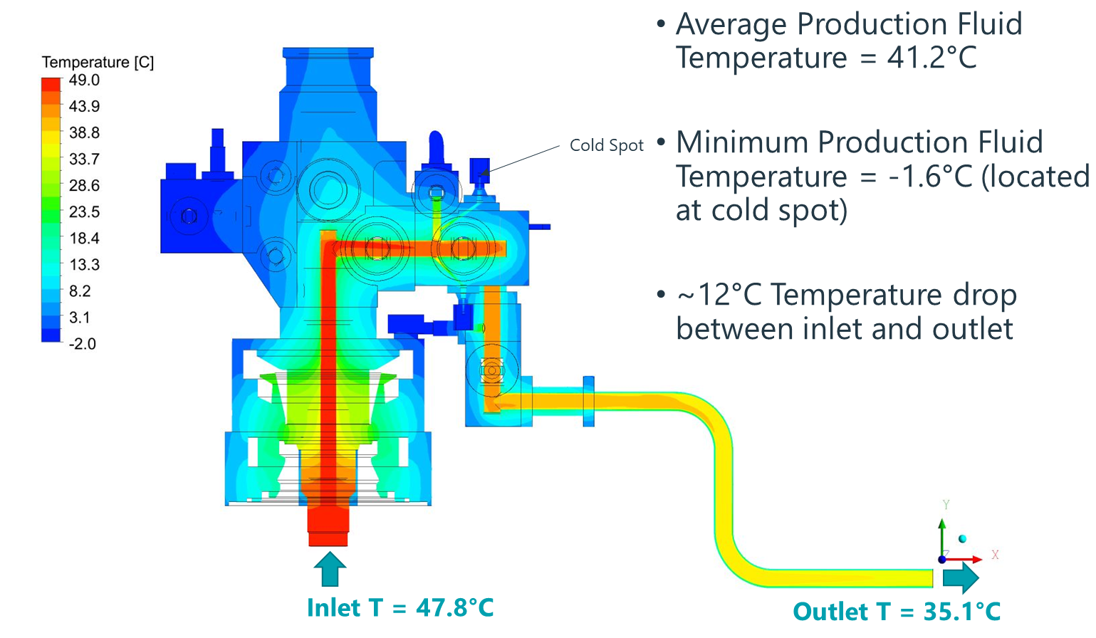
What we can see in the image above is a temperature contour of the steady state result for the tree (with no insulation) and we found that, between the inlet and the outlet, the temperature was losing around 12 deg C and also identified cold spots within the domain which reached minus 1.6 deg C. The freezing point of this fluid was 26 dec C, which means that there could be potential hydrate formation within these areas even during steady state operations.

The plot above depicts the liquid volume fraction and, as you can see, in that same area we see the liquid and gas splitting and there's an accumulation of gas sitting in this block. The gas, because there is a dead leg region, is left to cool quickly and it ends up sitting around that ambient temperature.
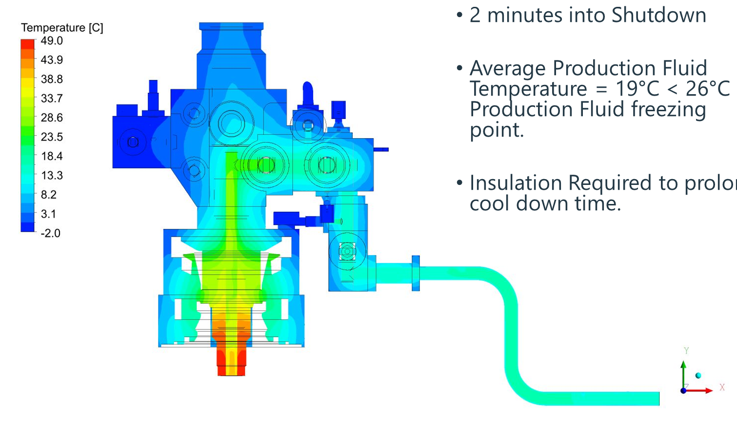
The picture above shows the temperature contour of the shutdown simulation at the two minute mark and what we can see is that the average production fluid temperature has fallen below 26 degrees which is below our designated production fluid freezing point. This means that this design did not satisfy the three-hour cool down time that we were designing to. Based on this, we knww straight away that insulation was required for this configuration to achieve the required cool down time.
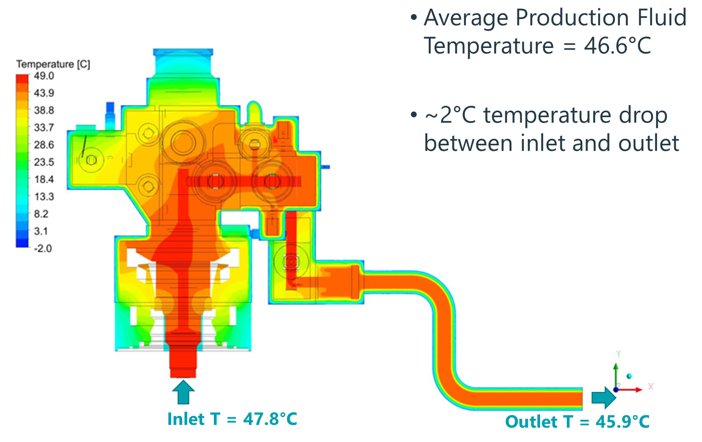
To confirm the level of insulation, we simulated scenarios that represented a series of different insulation thicknesses – in the image below you can see the results for the final insulation thickness that we used (2 inches of insulation surrounding the tree). This scenario showed greater heat retention within the body of the tree during steady state operations, and that temperature drop between the inlet and the outlet has fallen from around 12 degrees to only 2 degrees during steady-state operations. Also, the cold spot previously identified during steady-state operations in the dead leg has now disappeared.

And finally, the image above shows the shutdown temperature contours at the three hour mark, when using 2 inch insulation. It was found that the average production fluid temperature at this point was 26 degrees which means that the 2 inch insulation is sufficient to satisfy our requirement of cool down time within three hours, as shown in the video below:
For more information on Wood Group, please visit their website here.


