
In Part 2 of this blog series on Y+, we saw how the front wing flaps were not prone to separation under the given flow conditions. In Figure 14, the geometry was adjusted, and the flow was solved using meshes with y+ ~ 1 (above) and y+ ~ 30 (below). The velocity contours below show the first flap separating for the y+ ~ 1 case, changing the flow structure.
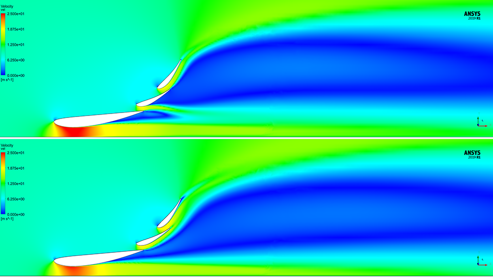
Figure 14 – Velocity distribution on the symmetry plane
The static pressure is lower for the y+ ~ 1 case around the main section, as shown in Figure 15.
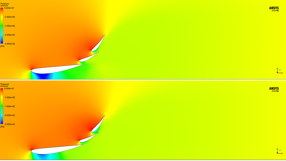
Figure 15 – Static pressure on the symmetry plane
This can also be seen in the static pressure plot for the main section in Figure 16.
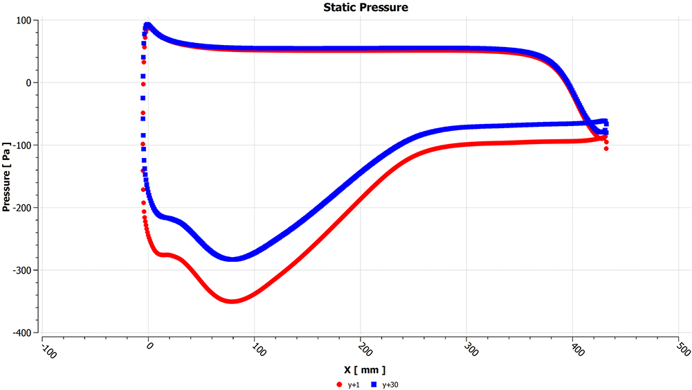
Figure 16 – Static pressure on the main section
The lift coefficient normalised using the y+ ~ 1 results given in Table 2 shows a 9% difference.
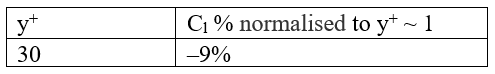
Table 2 – Lift coefficient normalised by y+ ~ 1 results.
This case shows that sensitivity is case dependent. It is therefore important to test each case for sensitivity.
Number of prism layers required to resolve the boundary layer
With a better understanding of the boundary layer in Part 1 and the effect of y^+ in Parts 2 and 3, the next question is how many prism layers are required to resolve the boundary layer?
One of the methods to evaluate if the boundary layer profile has been captured is to display the turbulent viscosity ratio: read more about it: Click Me
For problems with complex geometries and multiple surfaces growing different sized boundary layers, it may be required to run multiple simulations and vary the number of layers. In Part 4 we will look at applying the first layer sizing to fit a y+ ~ 1 near-wall layer and then vary the number of prism layers, monitoring forces.
Figure 17 shows different meshes created with different numbers of layers: 15 layers (top left), 20 layers (top right), 25 layers (bottom left) and 30 layers (bottom right).
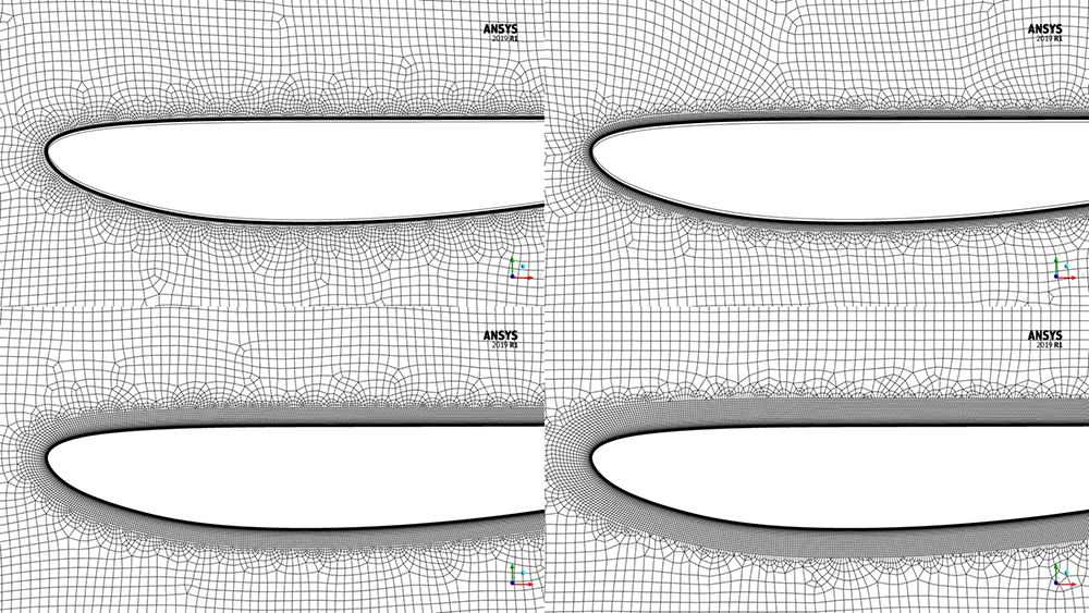
Figure 17 – Meshes with 15 layers (top left), 20 layers (top right), 25 layers (bottom left) and 30 layers (bottom right).
Figure 18 shows the corresponding plots of the turbulent viscosity ratio (TVR) for each of the meshes shown above. To properly resolve the boundary layer, the results should show that the ratio transitions from a low to high value and back again inside the prism layers. In this case, it can be observed by transitioning from blue to red and then green. The 25 and 30-layer plots show a clear transition, indicating the local boundary layer profile has been resolved. It is important to note this is not all that matters. In a real case, the number of layers that may resolve a front wing may not resolve the rear end of the diffuser that has seen 2 m of boundary layer growth.
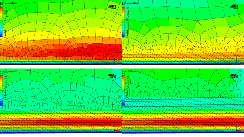
Figure 18 – The TVR distribution across the boundary layer for the four different mesh types
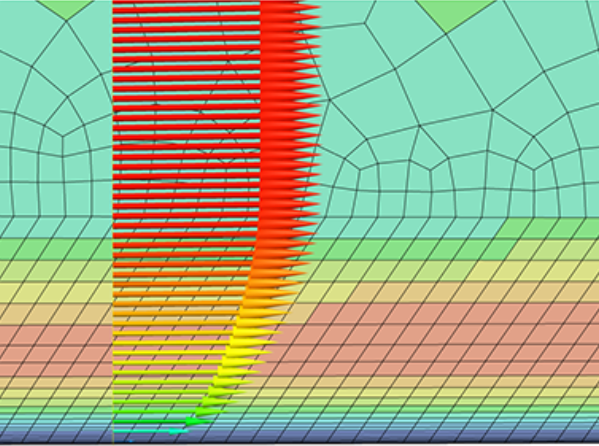
Figure 19 shows the turbulent viscosity ratio overlayed with velocity vectors, showing the different regions and how they are resolved.
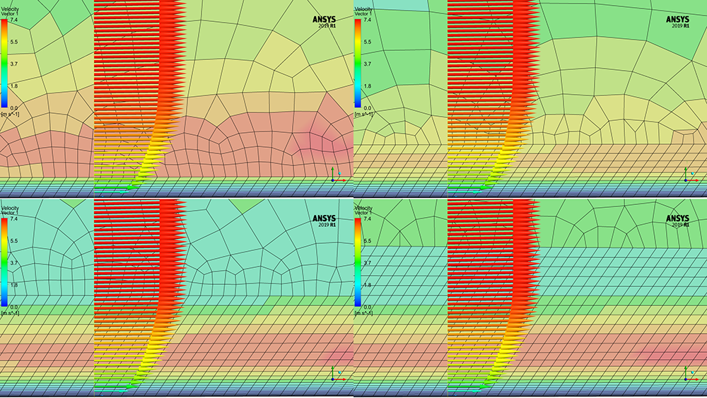
Figure 19 – TVR contours overlaid with velocity vectors on the different meshes
The boundary layer profile, towards the trailing edge of the main section, along the red line, is shown in Figure 20. The 25- and 30-layer cases are very similar with deviation shown in the other two. This shows that even with the first cell height being the same, without resolving the full boundary layer, the effect of the adverse pressure gradient changes the velocity profile.
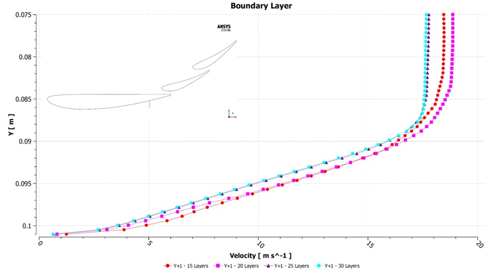
Figure 20 – Velocity profile on a line normal to the surface at the back of the main profile
Looking at wall shear stress distribution, shown in Figure 21, and zooming in on the end of the wing in Figure 22, the 20, 25 and 30 layer meshes separate around the same location, with 15-layer mesh deviating in the separation point by 30 mm.
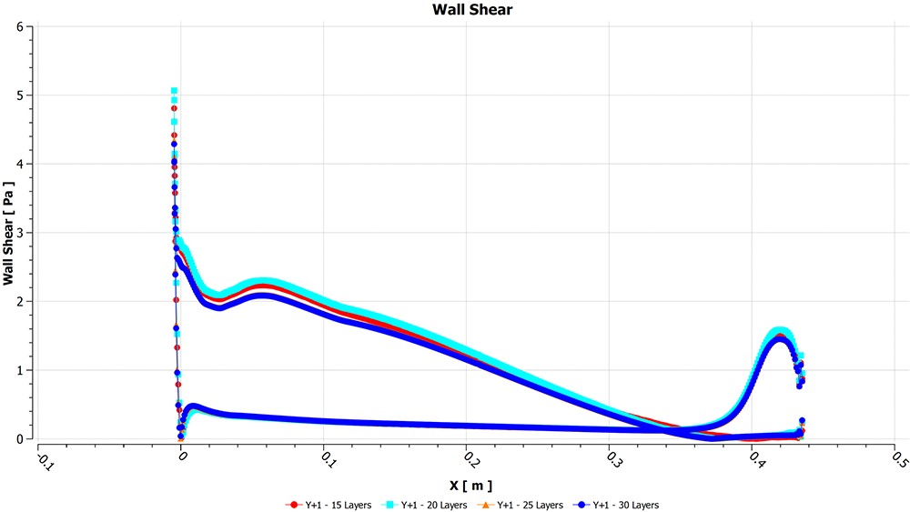
Figure 21 – Wall shear stress distribution on the main section
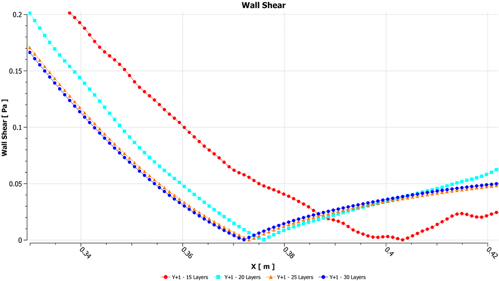
Figure 21 – Wall shear stress distribution on the main section
Static pressure around the main section is similar between the 25- and 30-layer cases, as seen in Figure 23. As the other cases are not accurately capturing the full boundary layer profile, they are not able to predict the effect of the adverse pressure gradient showing deviation.
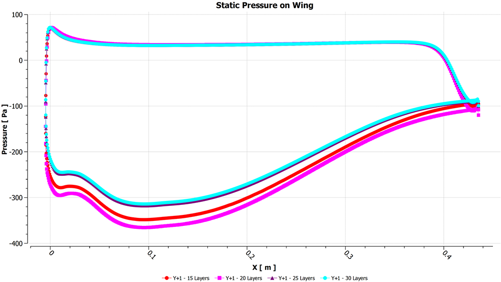
Figure 23 – Static pressure distribution on the main section
The lift (Cl) and drag (Cd) coefficient, normalised by the results obtained using 30-layers are shown in Table 3. There is a large variation of the forces if enough layers are not used to resolve the boundary layer. 25-layers show similar values, whereas the 20 and 15-layers show differences of 14% and 9% respectively in Cl.
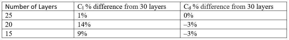
Table 3 – Lift and drag coefficients normalised by the 30-layers results
The question this four-part blog wanted to answer using a case study is: What value should I use in my simulations?
In Part 1, we looked at the underlying physics of the boundary layer and how it is modelled in CFD.
Part 2, used a 2D multi-section wing in ground effect mode to demonstrate the impact of using different values on the flow field, pressure distribution and wall shear stress around the main section, velocity profile on a line towards the trailing edge of the main section and force coefficients normalised to results. This demonstrated using a larger value large than 1 introduced modelling errors.
Part 3 showed what happened when the first flap was sensitive to flow separation. This demonstrated wall functions, under certain conditions, can underpredict flow separation, highlighting the importance of mesh sensitivity testing. We also examined the number of prism layers used to resolve the boundary layer for a case. Demonstrating how the flow field, pressure distribution and wall shear stress around the main section, velocity profile on a line towards the trailing edge of the main section and force coefficients normalised to the 30-layers case deviated. This highlighted why it is crucial to ensure enough layers are used to capture the boundary layer.
With all this information, you are probably thinking, “How can I apply this to my simulation?”
This is what I would recommend:
- Start with a 2D geometry of a component like the front wing
- 2D simulations are a great starting place, simulation run times are low, allowing for lots of testing, but flow features are inherently 3D, so force coefficients are not accurate.
- Run test cases for different values and prism layers. Reading about it is essential, but always test on your component.
- You can also use the 2D case to understand the effect of varying surface and volume mesh densities.
- As this blog has demonstrated, create a clear plan, change one variable at a time and review the results.
- The 2D results should give you an idea about the trade-off between accuracy (values, number of layers, force coefficients), and computational resources (simulation run times and RAM requirements).
- Create a simplified front wing in 3D in different conditions, i.e. straight line, pitch, roll and yaw
- Test different values and number of layers recording force coefficients, computational resources and review the results for each condition.
- cases resolve the viscous sub-layer, requiring a fine mesh, leading to longer run times which means fewer designs tested within a year.
- cases use wall functions, allowing for a coarser mesh, leading to shorter run times which means more designs tested within a year.
- After you are happy testing on a simplified model, apply your mesh settings to your full car in different conditions
- You may need to tweak your mesh settings as the number of prism layers required to resolve the boundary layers of a front wing and diffuser are different!
This concludes Part 3 in our series on 'What Y+ should I use?', you can refer back to the other parts in this series below:
- Part 1 – Understanding the physics of boundary layers
- Part 2 – Resolving each region of the boundary layer
Thank you for taking the time to read through this blog. If you have any comments or questions, please leave them in the comment section.


